Laser beam fine focus analyzer

 

 

 

 

 

 

 

 

 

 

 

 

Darmin Catak – s011480

 

David Bue Pedersen – s031950

Preface

 

 

First and foremost we would like to acknowledge The Department of Manufacturing Engineering, the Technical University of Denmark, and CALM without whom this project would not be possible.

 

CALM is an abbreviation of Centre for applied laser micro manufacture, and the experiments within this project have been conducted in laboratories provided by CALM and IPL (Department of Manufacturing Engineering) at DTU (Technical University of Denmark). The laser used for the experiments is a fiber laser also provided by the Institute of Mechanical Engineering and Manufacturing, built by NKT research, also a CALM partner.

 

As well as providing the laser and laboratory, they have provided us with the necessary finances and all other equipment that has been needed to conduct the experiments and build our device.

 

Also we would like to thank Mr. Peter Carøe Nielsen, Mr. Jacob Nielsen and professor Mr. Fleming O. Olsen for their supervision and patience during the creation and completion of this project.

 

We would also like to thank Peter, Jakob and Flemming for giving us the opportunity to undertake this interesting project, and for providing us with the necessary literature and materials needed to understand and grasp the task that was given to us.

 

 

 

Denmark, Kgs. Lyngby, January 31 2007

 

 

 

______________________ ____________________________

Darmin Catak – s011480 David Bue Pedersen – s031950

Abstract

 

A method for monitoring and analyzing a laser beam is being researched. In this report one will be presented with the challenging task and the considerations that must be taken in order to monitor and construct a tool for analyzing the laser beam from an industrial laser.

 

Based on a known method presented in the 1983 by Lim G.C. and Steen W.M, Dept. of Metallurgy, Imperial College, London SW7, GB, it will be shown that it is possible to monitor a laser beam with a high resolution using a relatively simple approach.

 

Though this method back in 1983 was proven to provide inline feedback in the form of a beam intensity profile, the method was at the stage of discovery suffering from the lack of tools for strong numerical data processing and data logging.

 

Today these tools are readily available at an affordable price. An improved analyzing method based on the method of 1983 will be examined through a series of experiments. These will serve as a reference in the final development of a laser beam analyzer.

 

By using off-the-shelf electronic components a simple, yet advanced control system as well as driver software for the beam analyzer will be created which will aid in collecting analytical data through experiments. This will result in much better and more accurate datasets, than what is possible to achieve by collecting analytical data manually.

Through extensive mathematical analysis using numerical mathematical tools there will be developed a script based on existing source provided by Mr. Peter Carøe Nielsen. The script will be written in MatlabÒ by MathworksÒ and will have the ability to automatically process data from the analyzer during experiments.

 

This data processing procedure gives a good picture of how the laser beam propagates. These data then serve as an aid in the monitoring and assessing the quality of the laser beam.

 

Furthermore a mechanical structure will be created. It will contain all the subsystems the analyzer is made of. It will provide the ability to measure the laser beam from different angles around the path of propagation, and it will be designed in a manner so that it can be used to measure most industrial or experimental lasers.

 

The laser beam analyzer will be designed with ease-of–use in mind so that it can be operated after a short introduction. It will be able to be connected to any personal computer, and it will be able to execute measurement series unassisted by a human operator, thereby eliminating a possible source of error.

 

Finally the construction of the laser beam analyzer will be expected to be much cheaper in comparison to the purchase of most existing laser beam analyzers on the market today.

 

Table of contents

Preface........................................................................................................................... 1

Abstract.......................................................................................................................... 3

1. Background................................................................................................................ 7

2. Project definition......................................................................................................... 8

3. Main objectives.......................................................................................................... 8

4. Theory...................................................................................................................... 10

4.1 The beam analyzer explained............................................................................ 10

4.2 An introduction to laser optics............................................................................ 11

5. The Laser platform................................................................................................... 14

5.1 The 20 W fiber laser........................................................................................... 14

5.2 The Optical system............................................................................................ 15

5.3 The NC system.................................................................................................. 15

6. Initial experiments:................................................................................................... 16

6.1 Experimental setup............................................................................................ 17

6.3 Initial experimental considerations:.................................................................... 17

6.4 Resolution parameters:...................................................................................... 17

6.5 Theoretical minimal rotational speed.................................................................. 20

6.6 Equipment used................................................................................................. 22

6.6.1 The DC motor:............................................................................................ 22

6.6.2 The reflective rod and fitting........................................................................ 22

6.6.3 The detector................................................................................................ 22

6.6.4 The beam dump.......................................................................................... 24

6.6.5 The vision system....................................................................................... 24

6.6.6 The oscilloscope:........................................................................................ 24

6.7 Other equipment used during the initial experiments......................................... 25

6.8 Experimental approach...................................................................................... 26

6.9 Experimental procedures................................................................................... 26

6.10 Commonly routines and commonly used parameters:.................................... 28

6.11 Experimental overview:.................................................................................... 29

6.12 Experiment 1:................................................................................................... 30

6.13 Experiment 2:................................................................................................... 31

6.14 Experiment 3:................................................................................................... 31

6.15 Experiment 4:................................................................................................... 32

6.16 Data post processing....................................................................................... 34

6.16.1 Needed data.............................................................................................. 34

6.16.2 Determining the Gaussian........................................................................ 34

6.16.3 Calculating the beam propagation path..................................................... 37

6.17 Presentation of data from the initial experiments............................................. 39

6.17.1 Experiment 1............................................................................................. 39

6.17.2 Experiment 2............................................................................................. 41

6.17.3 Experiment 3............................................................................................. 45

6.18.4 Experiment 4............................................................................................. 46

6.18 Conclusion of the initial experiments................................................................ 47

7 Designing the beam analyzer................................................................................... 49

7.1 The first design concepts:................................................................................. 50

7.2 The final design:................................................................................................. 53

7.2.1 The turntable and horizontal plate............................................................... 53

7.2.2 The ball bearing unit.................................................................................... 54

7.2.3 The back plate............................................................................................ 56

7.2.4 Reflector rod holder.................................................................................... 56

7.2.5 The reflector rod......................................................................................... 58

7.2.6 The inverted T-frame skeleton................................................................... 59

7.2.7 Spindle and linear motion rail....................................................................... 59

7.2.8 Strength of the turntable plane.................................................................... 60

7.3 Electronic components and mechatronics........................................................ 63

7.3.1 The power supply....................................................................................... 63

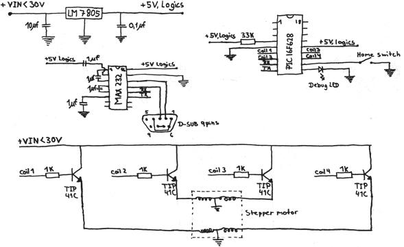
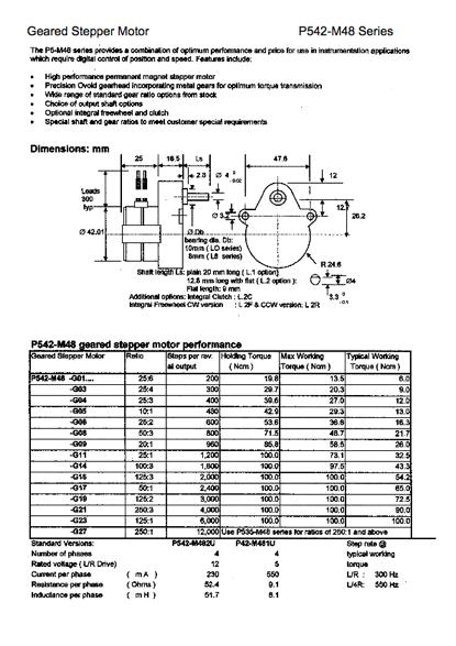
7.3.2 Stepper motor............................................................................................. 63

7.3.3 Stepper motor controller............................................................................. 65

7.3.4 Brushless motor and controller................................................................... 68

7.3.5 Beam analyzer controller software:............................................................ 70

7.3.6 REV counting mechanism........................................................................... 73

8 The finished laser beam analyzer............................................................................. 75

9 Economic overview................................................................................................... 77

10 Validating the laser beam analyzer......................................................................... 77

10.1 Measurement set 1.......................................................................................... 77

10.1.1 Measurement data 6A:.............................................................................. 78

10.1.2 Measurement data at 5.5A........................................................................ 80

10.1.3 Measurement data at 5A........................................................................... 82

10.2      Conclusion of the validation experiments.................................................... 84

10.3 Hunting the distortion problem......................................................................... 85

11 Error identification................................................................................................... 87

11.1 Human errors................................................................................................... 87

11.2 Reflector rod.................................................................................................... 87

11.3 Rotational speed.............................................................................................. 87

11.4 Cladding mode................................................................................................. 87

12 Conclusion.............................................................................................................. 89

13 Future work............................................................................................................. 90

14 References............................................................................................................. 91

15 Appendices............................................................................................................. 92

15.1 The documentation CD-ROM.......................................................................... 92

15.2 Matlab script..................................................................................................... 92

15.2.1 Gauss_fit.m............................................................................................... 92

15.2.2 beam_propagation.m................................................................................ 95

15.2.3 Support functions for the matlab script..................................................... 95

15.3 Stepper motor controller schematics............................................................... 97

15.4 Stepper motor controller firmware code.......................................................... 98

15.5 Stepper motor data sheet.............................................................................. 102

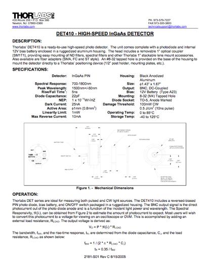
15.6 Detector datasheet........................................................................................ 103

15.7 SKF 61819 ball bearing datasheet................................................................. 104

15.8 Parts and costs.............................................................................................. 105

15.9 Technical drawings........................................................................................ 107

15.9.1 Turntable overview................................................................................. 107

15.9.3 Back plate............................................................................................... 108

15.9.3 Turntable plate........................................................................................ 109

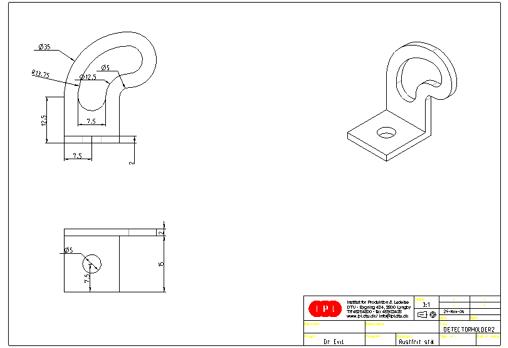
15.9.4 Reflector rod fitting.................................................................................. 110

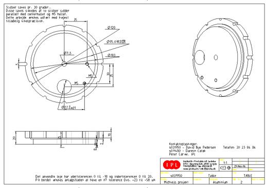
15.9.5 Turntable................................................................................................. 111

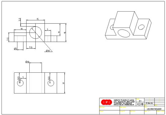
15.9.6 Detector holder....................................................................................... 112

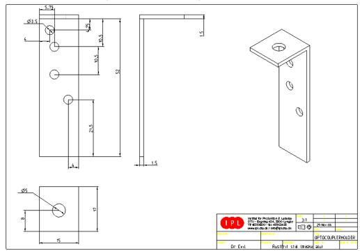
15.10 Optocoupler holder.................................................................................. 114

15.9 Tolerance chart.............................................................................................. 115

 

1. Background

 

 

In 1983 an article describing a laser beam analyzing method was published^[1]. The force of the method seemed to be the simplicity of the experimental setup and the ability of monitoring the intensity profile and spot size of a high power laser directly in the focus of the laser beam.

 

 

When using high power laser beams for industrial or research purposes it is very important that the process is monitored either in-process or offline.^[2]

 

Depending on the laser process, different characteristics of the beam itself need to be maintained. For example in laser welding or cutting, it is needed that the beam penetration is very narrow and deep. To make sure this is possible a finely formed beam with large depth of focus is needed.^[3] This is just one of the processes that requires monitoring, to make sure that the quality of the process, in this case the weld or cut, is kept. In other processes different characteristics are needed, but the monitoring is still very important if the quality is to be insured.

 

General perception of the laser beam is that its profile always stays constant, and that the laser system will always produce perfectly coherent results. However this is not true. Also written in the 1983-article is mentioned that it has been proven that if this consistency is to be kept then frequent analyzing of the beam is needed.

 

The basic principles behind the beam analyzing method and the optics involved will be further explained throughout the report.

2. Project definition

 

            The project forming the foundation for this rapport has the purpose of developing a beam analyzer that can measure the beam propagation of an industrial or experimental fiber laser.

 

The laser beam analyzer must be based on the principles described in the article from 1983 ^[1]. The final goal is to be able to describe a series of beam parameters such as parameters that describe the beam propagation path, and the intensity distribution over the beam.

 

            To construct the measuring equipment following work must be undertaken:

 

-      The underlying theory must be understood. This theory will form the knowledge base of the math and physics that will be used throughout the project.

 

-      Replication of the experimental setup from 1983 is needed for a proof-of-concept, and these initial analytical data will be used to define the further design requirements for the beam analyzer.

 

-      A data processing method will be developed. This will consist of the development of a numerical MatlabÒ script that will be used to process data from the beam analyzer.

 

-      A prototyping phase will be undertaken where possible beam analyzer designs are examined after which a final design is to be selected.

 

-      The manufacturing of the parts used in the beam analyzer will be ordered. Some parts is produced by the project team, and assembly of the laser beam will be undertaken.

 

-      Experimental work on the developed beam analyzer will be done for validation.

 

-      Finally the project will be documented in the form of the report you are currently reading.

 

 

 

 

 

 

3. Main objectives

 

 

The main objective of this project is to be able to measure the spot size at the focal point for lasers with a spot size down to of 10 µm. Only one geometrical binding has been requested by the IPL/CALM group. It is that the beam analyzer must be able to fit underneath a laser system with 50-70 mm clearance from the substructure to the laser nozzle.

Finally the beam analyzer must be developed with simplicity in mind and the budget of the laser beam analyzer must not exceed 2,000 $

 

Experiments conducted in the preliminary experimental work will define further demands and requirements that need to be abided for the beam analyzer to perform as desired. Final tests on the finished beam analyzer will show if these demands have been met.

 

 

 

 

 

 

 

 

 

 

 

 

 

 

 

 

 

 

4. Theory

 

            After a brief explanation of the working principle of the laser beam analyzer, the theory and optics that is used throughout the report will be explained

 

4.1 The beam analyzer explained

 

            The mechanism of the laser beam analyzer described in the 1983 article^[1] is very similar to what is seen in a supermarket bar-code reader. A laser beam is by a mechanism scanned over a detector. The detector delivers an output voltage representing the intensity of the light hitting the detector window. A barcode reader uses the intensity peaks received between the black lines in the bar code to read a binary code. The laser beam analyzer uses the output signal to measure the intensity distribution of the laser beam.

 

In a barcode reader a low powered laser diode < 5 mW are scanned over the barcode by a rotating mirror, and it is the reflections from the barcode that provides the signal. In the laser beam analyzer, the laser beam is reflected by a highly reflective rod rotating at high velocity trough the focus of the laser beam. As the rod travels trough the laser beam it is scanned directly over the detector that reads the intensity profile of the signal.

 

4.2 An introduction to laser optics

 

The model that most people have in mind when thinking of optics is a very simplified model descending back to childhood experiences with a magnifying glass used to focus the sunrays. The model states that a parallel bundle of sunrays are focused in an angle defined by the lens and that there is one clearly defined focal point in where the area of the beam spot is close to zero. This model is extremely simplified compared to what happens in reality. Light from a laser never propagates truly parallel, and diffraction sets a limit on how small a spot can be focused^[4].

 

The beam close to the focal point has the shape seen on figure 4.1. The beam waist is defined as the smallest radii of the beam throughout the path of propagation.^[5] Even though this is called the focal point, it is easily seen that the beam radii changes slowly close to focus, and that the intensity of the beam in this area is almost as high at the waist position. This focal range is also called the Rayleigh Length^[6].

 

The following optical parameters will be discussed:

            Beam waist:                [w₀]

            Rayleigh length:                      [z_r]

            Angle of divergence:   [q]

            Beam quality:              [M²]

 

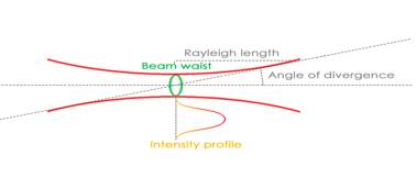
Figure 4.2.1 profile of the laser beam

 

 

 

Another common statement is the fact that a beam can be parallel. There is no such thing as a parallel beam. A beam bundle that starts as being parallel will further down the beam path slowly diverge due to diffraction. Diffraction is the phenomenon that a parallel beam bundle will spread as it propagates, much like the phenomenon that occurs when observing the backscattered waves as they roll back in a spreading formation after a wave front hits an offshore structure in the water. Furthermore there is a relation between wavelength and diffraction. For shorter wavelengths the diffraction is decreased.^[7]

 

The diffraction phenomenon is linked to another important parameter: The angle of divergence. This angle explains how hard the laser beam is focused and is defined from classic ray tracking. A hard focused beam has a high angle of divergence, and can focus to a smaller spot size than a beam with a smaller angle of divergence. The limit for how hard a laser beam can be focused is called the diffraction limitation phenomena^[8].

 

The parameters described so far can now be used to describe one of the most important parameters in the world of lasers. This is the M² value^[9]. This value is defined as the parameter for quantifying the beam quality of laser beams, and its form is seen in formula 4.1:

 

(Formula 4.2.1)

 

Where [q] is the angle of divergence, [l] is the wavelength of the laser and [w₀] is the beam waist.

 

 

The relation between M² and beam quality is that for higher quality M² ® 1. This can be explained in the following way. Assume that there are two lasers. Laser #1 with M² ≈ 1 and laser #2 with M² ≈ 2. They must be focused to the same spot size with same diameter of the focus lens. To obtain this, laser #2 must be focused harder than laser #1 This affects the position of the waist as it will be moved closer to the lens for laser #2 than laser #1.

 

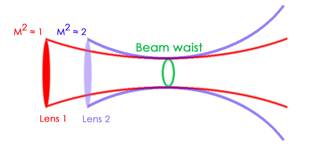
Figure 4.2.1 The relation between beam focusability and M²

 

 

Finally the Rayleigh length will be defined. The Rayleigh length is the distance from the beam waist at which the mode area is doubled. This is expressed with the following relation^[6]:

 

  (Formula 4.2.2)

 

Where [w_r] is the waist at the Rayleigh length and [w₀] is the beam waist.

 

The Rayleigh length for a diffraction limited optical system is given by the expression:

 

     (Formula 4.2.3)

[z_s] is the Rayleigh length, [w₀] is the beam waist and l is the wavelength.

 

 

If it is assumed that M² equals 1, the mode of the beam is a pure TEM00 mode.^[10] This means that the beam spot has the shape as seen on figure 4.3.

 

 

Figure 4.2.3 The shape of a TEM00 beam spot

 

 

The TEM00 mode is called the fundamental mode. The intensity profile across this mode is characterized by being a Gaussian distribution. For higher order modes this does not apply but the lasers used during all the experimental work which forms the basis of this thesis have a small M² value, almost a TEM00 mode and hence a close-to-Gaussian intensity distribution^[11].

 

The theoretically intensity profile for the fiber laser that was used during the experimental work is shown in the lower part of figure 1. It is a Gaussian distribution^[11] following formula 4.4:

 

       (Formula 4.2.4)

 

 

            Where the constants are real as well as: a > 0, b, and c

 

 

 

This completes the optical theory used within the thesis and will be referred to when needed.

5. The Laser platform.

 

5.1 The 20 W fiber laser

 

 

            The test subject in throughout the project is a mid-range 20 W fiber laser. This is suited and used for a wide range of experimental work. It is built into a safety cabinet making it a class I laser system, which means that anybody with a short briefing can use this laser.

 

20 W describes the maximal output power of the laser. Though 20 W isn’t much compared to high-power lasers this laser is far from weak when it comes to power density as the pure mode of the laser gives great focusability^{[figure 4.2.1].}

 

The determining factor for the quality of the fibre lasers are the type op fibre used in the laser. Single mode fibre lasers are known for a very pure and good mode because the output fibre only allows one mode to travel trough. This gives an unmatched M² and makes the beam easy to focus.

 

Specifications provided by the manufacturer^[12]:

            CW Ytterbium doped fiber module

            5-20W output power

Max current 6 A

Effect/Current rating of 3.47W/A.

            Single mode fiber delivery

Diffraction limited output

M²< 1.1 (The CALM laser is a prototype hence M² < 1.2)

Power vs. input current is linear.t

Fixed central wavelength between 1060-1090 nm (The CALM laser has been measured to 1075 nm)

 

 

 

5.2 The Optical system

 

 

            The optical delivery system consists are built up a follows: A SMA connection connects the output fiber from the laser to a collimator. The beam leaves the fiber as it propagates towards infinity at a at a known widening angle. At a desired width the beam are collimated. The Collimator is a convex lens as seen on figure 5.2.1, that is used to redirect the beam so it propagates in a close-to-straight path and the distance from the fiber to the collimating lens is the focal length of the collimating lens^[13].

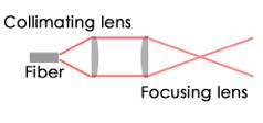
Figure 5.2.1 Optical system

 

When the beam is collimated it is ready to be focused. This is done by the focusing lens. The specifications of the optical system used is as follows:

 

-      Collimator: Focal length = 35.9 mm (red light), The diameter is oversized.

 

-      Focus lens: Focal length = 75.0 mm (red light), The diameter is oversized.

 

 

-      Estimated minimum waist: 8-9 mm

 

 

5.3 The NC system

           

            The laser is mounted in an NC setup. It is a 3 axis system with movement in the vertical and horizontal plane.

 

The NC table has two vertical axis called X and Y and a horizontal axis called Z. The X- and Y-axis are combined in a base structure and the Z axis is placed on a frame above the former axes. An overview can be seen on picture 5.3.1

 

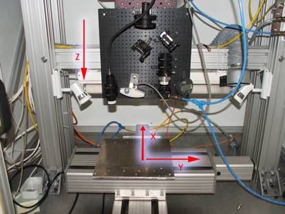
Figure 5.3.1 Axes of the NC system

 

The resolution of the NC setup is relevant since initial testing will rely on the resolution of all the axes. The resolution is seen in table 5.3.1.

 

Table 5.3.1 Resolution of the NC system.

 

The NC software used to control both laser and the NC system has its origin as a milling NC software. It has been adapted in such a way that the commands used to control the movement of the milling tool spindle will be used to control the laser instead. Hence the spindle speed controls are used to control the power of the fiber laser.

 

            Due to the fact that many lasers are missing a horizontal axis a similar 1 axis NC control system may be implemented in development of the beam analyzer to accommodate the need for such an axis.

 

 

6. Initial experiments:

 

            Before development of the laser beam analyzer can be initiated it is necessary to replicate the experiments conducted in 1983. This is done in the CALM/IPL laboratory on the 20W fiber laser.

 

6.1 Experimental setup

 

The experimental setup is very simple. A thin highly reflective rod is connected perpendicular to the axis of revolution of a miniature DC motor.

 

The dc motor is set to spin in a path perpendicular trough the laser beam.

 

Finally a detector coupled with a multimode mode 800 mm fiber is placed at roughly a 45 degrees angle above the rod and motor in such a manner that the laser beam will be scanned over the detector.

 

Picture 6.2.1 shows this simple setup what is used in the initial experiments:

 

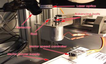
Picture 6.2.1 Initial experimental setup.

6.3 Initial experimental considerations:

 

            Lasers with different wavelengths as well as power density can be analyzed using the initial setup. There are three major areas of concern though.

 

The detector must be chosen to match the wavelength of the laser. The rod must be selected so that it reflects the wavelength. The speed of the rod must be so fast that the thread doesn’t take any damage by exposure from the laser beam, and hence the detector must have a rise/fall time that allows the needed rotational speed. A thorough explanation on this subject will be given in chapter 6.5.

 

6.4 Resolution parameters:

 

Related to the detecting mechanism is the diameter of the spinning rod, the area of the detector and its positioning in the respect to the plane of rotation of the rod. These are factors that will influence the measuring resolution of the arrangement. The governing equation for this^[1] is formula 6.4.1:

 

(Formula 6.4.1)

 

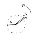
            The symbol explanation is as follows. r is distance from the rotational center of the rod to the measurement point. d is the diameter of the detector. l is the distance from the rod to the detector. q is the angle in which the detector is positioned. dx is the resolution. The different parameters are graphically represented in figure 6.4.1.

 

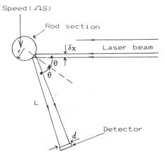
Figure 6.4.1 Parameters related to formula 6.4.1

 

           

            As the rod travels across the path of the beam, it will scanned over the detector which will give a response in form of an output voltage. This voltage corresponds to the beam intensity profile or power distribution. At any moment in time, the output voltage is proportional to the average power over an area defined by wδx where w is the length of the detector window in the direction of the length of the rod. This is visualized in figure 6.4.2

 

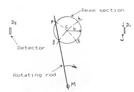
Figure 6.4.2 Graphical representation of wδx being the window of the detector

 

            The governing equation is not only useful for calculating the resolution but also very useful when defining an operational range. Knowing the resolution it becomes possible to optimize the other parameters being rod radius, measuring distance from rotational center, measuring angle and diameter of the detector window. By using simple mathematical algorithms one can generate a 3 dimensional graph in which one can find an optimal range of operation for any resolution. This means one can find a given set of parameters (r, d, l, and theta) for any known resolution, as seen on figure 6.4.3.

 

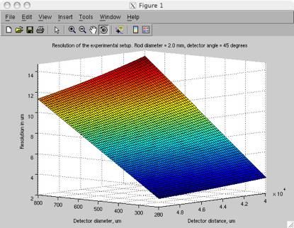
Figure 6.4.3 shows the resolution 3D graph

 

 

 

            This graph is made for a constant rod radius, and for a constant angle theta. It turns out that if one wants to manipulate all the parameters then the algorithm becomes more complicated, and the shear amount of data makes it difficult to present a visualization of the relations between parameters. Dark blue area is the area of interest for the experiments as this area provides the best resolution.

6.5 Theoretical minimal rotational speed

 

The speed of the rotation must not be too small or too great. If the speed is too small the laser will simply cut an indent in the rod. However if the speed is too great the detector, will not be able to sample the data correctly as it’s rise/fall time will be exceeded, and the true characteristics of the beam will not be known.

 

 

 

A lower limit of the rotational speed of the thread due to melting/vaporization damage to the thread can be calculated. This speed tells the user of the beam analyzer at which speed the thread should rotate on any given laser setup. The theoretical value will also be compared to experimental results found on the 20W fibre laser used for the experiments.

 

The following values are assumed:

 

            Laser: 20W.

Laser spot size: 0.03 mm radius.

Thread material: Aluminium

Reflector rod radii: 0.250 cm

Distance, measuring point - rotational centre: 3.5 cm

 

 

First of all the following material data for aluminium are used [www.matweb.com]:

 

 

Coefficient for light coupling into the material:

Thermal conductivity:

Heat capacity, solid phase:

Density:

Maximal allowed temperature:

 

Thermal diffusivity:

 

 

The maximal allowed exposure time for the thread with the given parameters can now be calculated from formula 6.5.1 which is derived from W. M. Steen, Laser material processing, third edition, formula (3.2).

 

            (Formula 6.5.1)

 

Where F₀ is the absorbed power density:

 

(Formula 6.5.2)

 

 

Now t_max can be found:

 

 

The minimal rotational speed can finally be calculated:

 

 

 

 

 

 

 

 

 

This theoretically lowest rotational speed are used as an indicator of how slow the reflector rod can rotate without taking damage

           

6.6 Equipment used

 

 

6.6.1 The DC motor:

 

            The DC motor used to rotate the thread was and OEM bulk DC motor with unknown specifications. The maximal rotational speed was well above 17.000 RPM though. The motor is fixated with a vise and positioned on the X-Y planes of the NC system.

 

 

6.6.2 The reflective rod and fitting

 

The reflective rod that is mounted on the DC motor is held in place by an aluminum fitting turned on a lathe in a student’s metal workshop located on Campus at DTU. A rough balancing mechanism has been built into the fitting so that it has a symmetrical plane through the axis of revolution. It can be seen in Picture 6.2.1. The reflective rod itself is cut of an aluminum TIG welding filler rod, since the coupling of the laser light into aluminum at a wavelength of 1075 nm is very low as seen on fig 6.6.2.1.

 

 

 

Figure 6.6.2.1 Reflectivity of rod material^[14]

 

6.6.3 The detector

 

 

The detector type is chosen depending on the wavelength of the beam, so that it matches the type of laser being analyzed. To solve this problem the simplicity of the device allows it to have an indefinite range in regards to the detectors, by simply interchanging the fiber attachment to the detector.

 

The detector used during the experimental work has been produced by Thorlabs and has the following specifications:

 

Detector: InGaAs PIN

Housing: Black Anodized Aluminum

Spectral Response: 700-1800nm

Size: φ1.43” x 1.67”

Peak Wavelength: 1500nm+/-50nm

Output: BNC, DC-Coupled

Rise/Fall Time1: 5ns

Bias: 12V Battery (Type A23)

 

            Further specifications can be found in appendix 15.6

 

Where it is the spectral response, peak wavelength, and rise/fall time that are the deterministic parameters that tells whether the detector is suited for any given laser.

 

 

 

6.6.4 The beam dump

 

A 1x80x100 mm sheet of copper is bent in a 45 degree angle so that it can be strategically placed beneath the experimental setup to diverge the laser beam, hereby minimizing the risk of backscattered light from the surroundings into the detector.

 

6.6.5 The vision system

 

A vision system is used for as guidance when the laser is positioned relative to the experimental setup. This system consists of a computer with a USB webcam, positioned on the Z-axis of the NC system, overlooking the experimental setup.

 

6.6.6 The oscilloscope:

 

 

            A Picoscope 3206, USB based oscilloscope is used to collect data from the detector. The same computer that drives the NC software and the webcam is running Picoscope 3206 through its driver- and monitoring software. This software gives the user the ability to capture datasets in a tab-delimited format which is cut n paste compatible with MS Excel.

 

 

 

6.7 Other equipment used during the initial experiments

 

An NC optical measuring device, the DeMeet, as well as a laboratory standard graded stereomicroscope has been used as well has been used to visually inspect the rod for vaporization damage and to check the surface roughness. Measuring tools as a Caliper Vernier and a micrometer clock has been used to set up the experimental rigging. A class I b, 4 mW red HeNe laser with a fiber coupling has been used to visually inspect the beam path throughout the experimental setup for alignment purposes.

 

6.8 Experimental approach

 

            The initial experiments to replicate the beam analyzing method from 1983^[1] was predominantly conduct to validate that the analyzing method. Some of the experiments though were conduct to validate theoretical calculations and theories such as the minimal rotational speed and the resolution calculations mentioned in chapters 6.5.

 

6.9 Experimental procedures

 

 

            The NC and fiber laser system are powered up. A reference run is executed to home all NC axes, and the NC system are moved to the desired position.

 

            A piece of aluminum TIG filler rod is cut and connected to the miniature dc motor via the axle fitting. The motor is bolted down to a plate, which is held in place by a vice grip. They are placed on the X-Y- NC plane directly beneath the laser optics. The dc motor is powered up and if needed the rod is balanced by adjusting its position in the fitting. The laser cabinet is closed, power output of the laser is checked and the laser is turned on. A small spot is seen on the vision system seemingly hanging in mid air as it hits the path of rotation of the rod as seen in picture 6.9.1

 

 

 

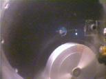
Picture 6.9.1 beam spot in mid air.

 

 

           The Z-axis are tuned so that the spot visually is as small as it can be focused. Hereby the focal point is determined very roughly.

 

The detector are coupled to a 800 micrometer fiber through an SMA connector and the far end of the fiber are connected to a tube formed black anodized aluminum shielding. The aluminum shielding is fixated to a tripod with a clamp and placed at a roughly 45 degrees above the rotating rod. For alignment purposes the procedure above can be executed with the red HeNe laser attached to the optics instead of the Fiber laser. Hereby tuning of the setup can be performed with the doors of the laser cabinet opened.

 

            Monitoring and measuring is performed by attaching the detector with a coaxial cable, and a 50 ohms terminator to the Picoscope. The Picoscope software interface is then ready to be used to capture sample data as tab delimited text.

 

6.10 Commonly routines and commonly used parameters:

 

For all experiments a few things must be determined for later use when the experimental data is being post processed. These are:

 

-      The horizontal offset from the focal point of the laser to the center of revolution of the motor.

 

-      The rotational speed of the miniature DC motor.

 

The following routines must also be performed before each experiment:

 

After a rough determination of the focal point, by using the method described in chapter 6.9, the horizontal position is trimmed by moving the X- and Y- NC axes while examining the detector signal intensity on the oscilloscope. This makes it possible to tune the X- and Y- axis so that the laser beam is placed where the signal is strongest. Now the laser beam is moved in the vertical direction (the Z axis) until the signal is strongest to determine the focal point more accurately.

 

When found, the laser is vertically placed so that the signal is strongest so that the focal point lies on top of the rod.

 

It is now time to determine the commonly used parameters. The rotational speed is first found. The Picoscope software is set up so the sampling range contains two signal peaks from the detector. The distance between these two peaks can now be measured. The value is noted so that it is available at post processing.

 

The other common parameter being the horizontal offset is now measured. The position of the NC table is noted. The NC table is moved so that the laser spot will hit the rotational center of the rod fitting. This is clearly seen as the fitting is turned on a lathe and therefore small groves in the surface from the machining process draws a spiraling pattern towards the rotational center. When the rotational center is found the new position is noted. By using trivial classical trigonometry the distance from the measuring point to the rotational center can now be calculated.

 

Finally the laser is moved back to the optimum signal position and the setup is ready to be used to conduct experiments. This position will in experiments 1-4 be reffered to as the initial position.

 

 

6.11 Experimental overview:

 

 

            Experiments of interest are as following:

 

1)    The collection of a data series by moving the laser in the vertical plane (NC z-axis) so that a beam propagation path can be calculated from the captured data.

 

2)    Two collection of data series where the NC table first is moved in the X- and then in the Y- directions to determine the sensitivity of horizontal positioning of the beam.

 

 

3)    The effects of the power variation of the laser by analyzing the detector output signal strength.

 

4)    A collection of data series from different detector viewpoints to determine if the beam propagation is symmetrical.

 

 

6.12 Experiment 1:

 

 

            The first experiment conducted is the variation of the vertical position of the laser. This was done to be able to calculate a beam propagation path and to see if it was possible to determine whether the optical system was not askew. It is also this experiment that will tell whether it is possible to replicate the experiments from 1983 on the experimental setup. The task is therefore to capture sufficient data to calculate the beam propagation. Sketch 6.12.1 shows a diagram of the setup.

 

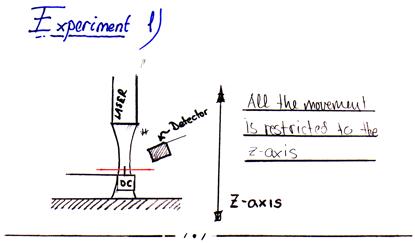
Sketch 6.12.1 Experiment one setup seen from side

 

 

The laser is placed in the initial position. The Z axis are moved down until the output signal of the detector is halved. This offset should place the focal point roughly the distance of the Rayleigh length above the experimental setup. The distance,- dZ, is noted

 

            Next is off course to perform a set of measurements. The laser is moved in its vertical plane. A step length calculated by using the vertical offset, dZ, is calculated by the equation: so that the measuring series are finalized when the horizontal offset is +dZ. For each step a scan over the detector is dumped from the oscilloscope to an MS Excel datasheet.

 

            The data is finally saved in a tab delimited text format from MS Excel so they are ready for the data post processing.

 

 

 

6.13 Experiment 2:

 

 

            Preparations positioning of the laser beam follows that for experiment 1. One must first align and then find the focal point. However it is of interest of this experiment that after finding the focal point that the laser remains stationary in the vertical direction. Instead the rod is moved in the horizontal plane. Sketch 6.13.1 shows a diagram for this setup.

 

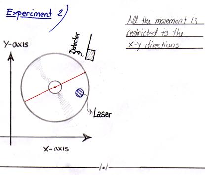
Sketch 6.13.1 experiment 2 seen from above

 

The laser is moved to the initial position. First the setup is moved in one direction e.g. the X direction until the intensity is roughly halved. Then the rod is moved to the original position and the experiment is repeated in the –X direction. This is also done for the Y direction. Data is dumped for each step, and the step length is determined as in experiment 1 so that 20 datasets are retrieved.

 

 

 

6.14 Experiment 3:

 

 

            This experiment is to conducted to examine the linearity of the experimental setup in relation to the laser output power. The laser output is according to the manufacturer linear and testsheets delivered with the laser proves this. By analyzing the output of the detector by varying the power of the laser it can be analyzed ehether the detector and the rest of the experimental setup behaves linearly as well.

 

The laser is moved to the initial postion. Then a set of measuring data is captured and saved in MS excel for varying power settings starting at the maximum power output. After data series is collected power is turned 500 mA down, and the data captured again. This is done in repetition until the output power of the laser has been halved. A sketch of the setup is also provided for this experiment in sketch 6.14.1

 

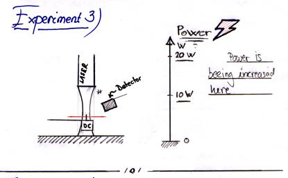
Figure 6.14.1 experiment 3

 

 

 

 

 

6.15 Experiment 4:

 

            This last experiment is done to see whether the beam path is symmetrical around the axis of propagation. The experiment is actually a repeating of experiment 1, after which the experimental rig is turned 90 degrees after which the experiment is performed yet again. When the experimental data is processed it will be possible to compare the two calculated beam propagation paths against each other hereby and determine any irregularities of the beam path that might exist.

 

 

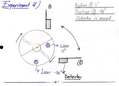
Sketch 6.15 Experiment 4 as seen from above

 

 

 

 

 

6.16 Data post processing

 

When a set of measurement data has been captured from the experimental setup it is necessary to perform several steps in a data post processing procedure. This will be carried out in MatlabÒ by MathworksÒ. This chapter describes how a beam propagation calculation is performed as in experiment 1 and 4 since this is the way the post processing will be performed when the final beam analyzer is constructed and a beam propagation profile is measured. Post processing of data in experiment 2 and 3 is done by only applying a certain part of the procedure described below namely the fitting of the captured data. A captured dataset describes the intensity profile through the beam and since this is assumed to be a Gaussian distribution for the fiber laser it is therefore fitted to match this. The complete step-by-step beam propagation data post processing as for experiment 1are therefore described in a general fashion so that it is not limited to the laser setup at IPL/CALM.

 

6.16.1 Needed data.

 

First of all the following parameters has to be found:

           

            - Rotational speed of the rod.

 

- Horizontal offset from the measuring point to the rotational center of the rod.

 

- Wavelength of the laser, which can be assumed with reasonable precision.

 

 

The horizontal offset to the measuring point is best determined by using the lasers own horizontal NC plane if available. If measurements are performed on a laser that cannot translate in the horizontal plane, it is easy to determine the distance by powering off the miniature motor, and fixating a small sticky-note on the rotor. Now a small hole can be machined in the paper with the laser and the distance from the hole to the rotational center is measured with a Vernier caliper. Hereby the distance in mm. can be determined with at least one decimal.

 

6.16.2 Determining the Gaussian.

 

The sample data for a measurement series consist of several datasets measured with different vertical offsets relative to the assumed focal point of the laser. A dataset corresponds to a scan of the laser beam over the detector in a horizontal plane and is a two dimensional measurement in a vertical plane.

 

 

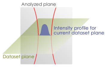
Figure 6.16.2.1 Overview of the planes of described in the procedure

 

Each dataset captured consists of a 2xn matrix where n represents the number of sample points in each dataset. The first column of data is the time in nanoseconds at where the data point was registered by the scope, and the second column is the signal voltage that describes the relative intensity of the laser at that point in time. This intensity is for fiber lasers expected to be a Gaussian distribution.

 

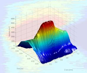
The raw source data are plotted as 3D and a 2D graph with color gradients representing intensity for the user to inspect before the matlab script continues. The picture below shows a beam propagation graph in 3D. As it clearly can be seen, applying different levels of smoothing and lighting effects can help during the inspection of the source data.

 

 

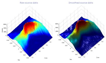
Figure 6.16.2.2 A 3D image of the beam propagation

 

 

After plotting the graphs, the time axis is converted to distance using the parameters of rotational speed and the distance from the measuring point to the rotational center. Hereby the intensity at the laser versus the distance from the center of the beam is known in all the datasets each representing a horizontal plane

 

As each dataset is expected to be a Gaussian distribution they are now being approximated with a nonlinear least-squares regression fitting algorithm that returns four deterministic constants for the Gaussian expression^[15]:

 

(Formula 6.16.2.1)

 

 

Where:

 

b₁ - is the relative intensity

b₂ - is the waist of the Gaussian distribution

            b₃ – is the offset

            b₄ – is the background/ the low signal

 

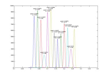
The outcome of the fitting procedure can be visualized graphically as seen in figure 6.16.2.3:

 

Figure 6.16.2.3 Raw source data with fitted Gaussian curves.

 

 

When the fitting algorithm has ended each dataset is now replaced by a Gaussian expression with varying constants and are saved to a text file on the computer containing a 5xn matrix with the first column containing the relative z-height, and the last four columns contain the above constants. This is done because the calculations so far are heavy to compute, and require full CPU time for several minutes. The rest of the calculations can at this way later be run separately to review the results of the calculaions.

 

 

6.16.3 Calculating the beam propagation path.

 

 

The data that was saved as output when the source data was fitted to the Gaussian expression is loaded. The first and third column of these source data being two 1xn column vectors containing the relative z height of the dataset and the waist of the Gaussian distribution are used to perform another nonlinear least-squares regression fit.

 

This time the Gaussian waist are interpreted as the beam diameter at a given z height, the sideways offset is normalized, and the fitting algorithm is performed on a formula that is derived based on another well known formula from laser optics. It is the formula that describes the beam diameter as function of the beam path.^[16]

 

The derived formula has the following appearance:

 

 

(Formula 6.16.3.1)

Where:

 

b₂ - is the beam waist (Smallest beam diameter)

            b₃ – is the M²

            b₄ – is the waist position

            l - is a constant containing the wavelength of the laser

z – Is an offset constant in the direction of the beam propagation as the formula requires that the y axis is placed at the beam waist.

 

When the fitting algorithm is finished, it returns the numerical determined waist and M² that matches the measurement data and finally a 2D graph is plotted that shows the beam propagation with the x-axis as symmetrical axis through the center of the beam path.

 

Figure 6.16.3.1 Beam waist and M²

 

 

           

6.17 Presentation of data from the initial experiments.

 

 

6.17.1 Experiment 1.

 

            Experiment 1 was intended to be a proof-concept experiment. Experimental data was processed by the MatlabÒ post processing algorithm.

 

It was shown that the experimental setup from 1983^[1] had been successfully replicated and that it was possible to calculate a beam propagation path with, M2 and the beam waist in mm.

 

Graph 6.17.1.1. Showing beam waist [mm], M2 value and propagation path.

 

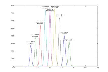
6.17.2 Experiment 2.

 

            This experiment was intended to show the influence of offsetting the experimental setup in relation to the laser. It was done to examine how important it is to align the beam analyzer correctly under the laser. The graphs below shows the Gaussian waist as well as the intensity (not to confuse of the beam waist) of data series sampled from the Picoscope. As the intensity of the signal in mV is a relative factor describing the energy distribution of the spot it is not as important as the Gaussian waist, which is needed to be roughly the some for the offset to be unimportant.

 

The first dataset to be presented are the data for variations in the x-direction. This corresponds to changing the measuring distance from the rotational center of the experimental setup.

 

Graph 6.17.2.1 Showing Gaussian fits with intensity [mV] in the vertical direction

 

A totally random intensity pattern is seen for the intensity signals. This seems to be related to the surface quality of the reflecting rod, where high intensity is obtained where the surface is even and low intensity is related to scratches and imperfections in the surface of the rod.

 

 

Since the intensity of the signal describes the intensity of the laser in a relative manner, this behavior might only to some extent affect the signal. Another important parameter is the waist of the Gaussian distribution that is used to describe the beam diameter. These values must not deviate as much and as randomly as is the case with the intensity. The Gaussian waist as a function of dX distance is plotted to observe this and as expected the waist is close-to constant. The added trend line shows a slightly falling beam waist as the measuring point are moved further out the rod. The falling tendency is only around one mm and more deep analysis must be performed the show if this is due to deviation or a true tendency.

 

Graph 6.17.2.2 The Gaussian waist as a function of X direction

 

 

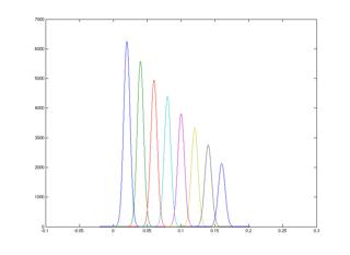
The same two graphs has been made for varying Y offset. This direction is perpendicular to the rod when it is struck by the laser light. If the measurement point is offset in this direction it will mean that the plane in which the reflected laser beam is scanned will be at an angle to the detector.

 

This can be critical when a fiber is used to collect the laser beam since a steep interaction angle to the fiber can result in what is known as cladding mode^{[Chapter 11.4]}. It will also affect the intensity of the collected signal and Gaussian waist as follows.

 

Graph 6.17.2.3 Showing Gaussian fits with intensity [mV] in the vertical direction

 

It is clearly seen that the intensity of the Gaussian waist is a function of Y offset and hence the interaction angle of the collecting fiber of the detector As with the X-series this can be ruled irrelevant and the most important analysis is if the beam waist is affected.

 

 

Graph 6.17.2.2 The Gaussian waist as a function of Y direction

 

The trend line again shows that there could be a rising tendency of approximately 1 mm. This cannot be ruled out to be deviation.

 

 

6.17.3 Experiment 3.

 

            This experiment, which is the simplest of the latter, was intended to show if the experimental setup behaved linearly in relation to lasing power. The fiber laser from the IPL/CALM behaves absolutely linear in relation to the applied current. By changing the output current of the laser it was therefore possible to see if the experimental setup had any unexpected nonlinear effects.

 

Graph 6.17.3. Signal intensity VS. power. Horizontal axis [mV]

 

The graph show the signal strength in mV with the intensity falling from full output power at 20W with a current decrease of 500 mA pr. step.

 

It is clearly seen that the experimental setup act linear and as expected that no nonlinear effects shroud cause worries throughout data processing.

 

6.18.4 Experiment 4.

 

 

            The final setup was intended to show if the beam propagated uniformly. Data captured from the experiment is shown below.

 

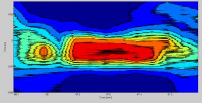
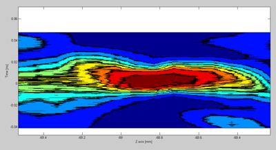
Figure 6.18.4.1 It is clearly seen that the beam propagates differently in the two planes

 

As seen on figure 6.18.4.1 the beam seems to propagate differently in the two planes. The beam waist can just from examining the raw data, be seen to differ from the two planes of investigation. This means that the measurement data tells us that the beam spot has an oval shape. The difference in z-axis values is due to the rearrangement of the setup and should be neglected.

 

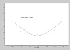
Figure 6.18.4.2 The beam propagation calculation. The difference in propagation path is obvious

 

The beam propagation paths for the two measurements also clearly shows a difference in the way the beam propagates throughout the planes. Due to the limited amount of data points is difficult to say whether the very two beam propagation calculations are so very different in reality of whether it’s a bad case of deviation. The difference is so big though that a difference in propagation pattern in the two planes in some degree must be to blame.

 

 

6.18 Conclusion of the initial experiments

 

 

            The method of beam analyzing from 1983 has been verified. Even more important is the fact that it has been proven that the method of beam analyzing from 1983 has the potential to be adapted and integrated to new and very strong numerical tools, when applied reveals much more information of the laser beam than what could be retrieved from the experimental data in 1983. Roughly speaking, it was only possible to monitor the intensity profile, compared to now where a full beam propagation path can be estimated.

 

Alignment sensitivity has been determined not to be to sensitive in both X- an Y- direction. A positioning with an accuracy of 0.1 mm seem be enough, and is an important factor in the upcoming design and development of the final beam analyzer. This means in other words that any NC based laser with an axial precision of 0.1 mm or better will be compatible.

 

Yet another great thing visible from the initial experiments is the fact that the system as a whole acts in a linear manner. This makes interpreting the experimental data much easier.

 

Finally it has been proven that it is possible to determine how the beam propagates through different cross sections of the laser beam. In experiment 4, the beam path at two perpendicular measurement points were held together to give a more detailed view of the laser beam. This method could be expanded to actually generate a 3D propagation graph based on data collected all the way around the laser beam.

 

 

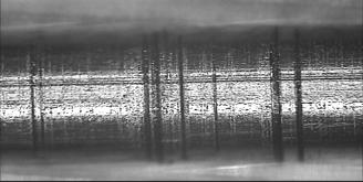
During the experimental work it was experienced that the miniature DC motor had to be run at its maximal rotational speed to avoid vaporization damage of the rod from the laser beam. The damage can easily be seen on picture 6.18.1, and needs to be addressed during the design of the laser beam analyzer.

 

Picture 6.18.1 Vaporization pattern, 10,000 RPM, Aluminum

 

It was experienced that a limiting factor throughout all the experiments was time. Collecting data manually took much longer time than expected which limited the amount of sample points and hence the resolution of the post processed.

 

This is another important discovery that must be addressed when designing the beam analyzer. It is of greatest importance that an automated data capturing process is developed. An experiment taking 2-3 hours to conduct could in best case be conducted in a matter of minutes if the entire process can be automated

7. Designing the beam analyzer.

 

 

The preliminary experiments have provided valuable experiences that will be used within the designing of the beam analyzer. The experiments define further demands and requirements that need to be abided for the beam analyzer to perform as desired.

 

These demands and requirements as well as the demands stated in chapter 3 was used to make a detailed system requirements outline.

 

The new set system specifications to be met are:

 

           

-       Capable of measuring spot size down to of 10 µm.

-       A horizontal measuring resolution down to of at least 1 µm.

-       Maximum 70 mm clearance from the substructure to the laser nozzle.

-       The analyzer must be able to collect data autonomous

-       The revolution speed range of the rod must be from 7000-40000 RPM to accommodate more powerful lasers than the one used for the experimental work

-       Inline monitoring module for motor RPM.

-       The replacement of reflector rod must be easy.

-       Vibrations in the structure must not be visible on measurements performed with a micrometer clock.

-       Budget must not exceed 2,000 $

 

Final tests on the beam analyzer after it has been built will show if these demands have been met.

 

 

7.1 The first design concepts:  

 

 

In the design phase one must consider following:

 

1)    Specification requirements

2)    How simple can the system be made

3)    What does the system need and what would just be nice to have in the system

 

With those factors in mind one can use a simple morphology table to create a series of possible solutions to the design. To create such a table, one must first identify the sub systems. The beam analyzer has for the morphological analysis been broken down to the following sub systems:

 

a)    Propulsion for the reflector rod

b)    Propulsion feedback

c)    Transmission

d)    The reflector rod(s)

e)    Vertical axis

f)      Propulsion for the vertical axis

g)    Detector system(s)

h)    Possible use of drivers and software

i)      Calibration aiming aids for the system

 

 

Only after these systems have been identified can a morphology table be created. Each system will have a number possible of solutions attached to it as seen on figure 7.1.1

 

 

 

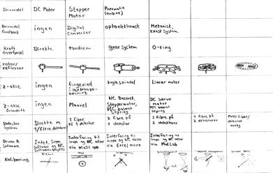
Figure 7.1.1 Morphology table

 

 

 

            What this table does is giving the developer the ability to create random solutions by going down the table and choosing what seem to be compatible subsystems.

 

Some of the more ore less random generated solutions will not be very good but most of them would comply with the specifications and do deserve a second look.

 

After narrowing the solutions down to 4 or 5, then one must look at the positive and negative sides of the solutions that are left. An good way of handling this so is to grade the solution and subsystems. The one with the highest overall score will likely be the final concept.

 

 

All subsystems of the candidate systems has been graded. Some of these subsystems are e.g. the reflector rod system, detector systems, the data collection rate, manually vs. automated alignment and calibration methods, their complexity, et cetera.

 

            The first concept was based on a box-like structure. It was possible to control the vertical movement by implementing a stepper motor control. Also it was sufficiently compact to be positioned underneath most lasers. A table would be moved vertically up and down and in the centre of the plate there would be placed a turntable on which would host a subsystem consisting of the reflector rod and motor. This turntable could be rotated so that the laser beam could be monitored from different angles. Figure 7.1.2 is a CAD generated image of the first concept.

 

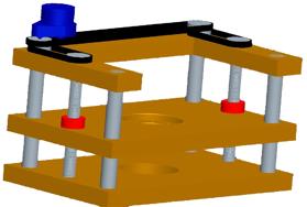
Figure 7.1.2 CAD drawing of concept no. 1

 

The system demanded two spindles. They would be required to turn at the same speed and at the same time a transmission of sort was demanded. A belt drive was the obvious solution since this would synchronize the two spindles.

 

            This concept was rejected though. The rods supporting the structure that also served as guide rods caused concern. The structure was designed like this to provide the most stable possible but if any of the four guide rods were to be misaligned it would potentially cause the whole system to get stuck. Also it was much to complex to build within the timeframe available.

 

            However some of the ideas found in the first concept are also to be found in the final concept. The central table, spindle, and the turntable for holding the detector/rod were kept. The way they were constructed and assembled can be found in the following chapters.

 

7.2 The final design:

 

The final design would be a scaled-down system similar to the previously presented rejected design. An inverted T-frame structure will be the structural skeleton and hold a linear rail an a ball screw spindle. Attached to these is a base plate that holds the analytical arrangement consisting of the reflector rod, rod motor, a fiber holder for the attachment of the detector and an optocoupler to count the revolutional speed of the rod. All part that needs to be manufactured will be made of aluminum alloy due its good machineability. All CAD drawings can be found in appendix 15.9 as well as on the documentation CD-ROM, appendix 15.1.

 

 

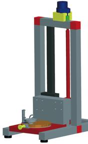
Figure 7.2.1 CAD drawing of the stepper motor controller

 

 

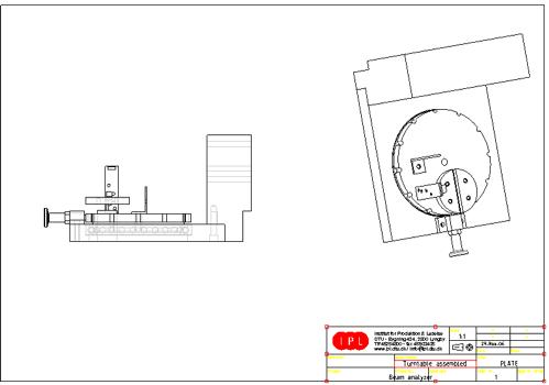
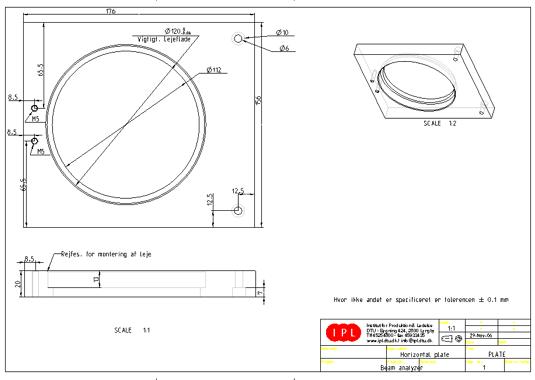
7.2.1 The turntable and horizontal plate

 

            For making 3D beam analysis the beam reflector and collector system is mounted on an NC milled turntable with a fixed 30 degree indexing system. This gives the beam analyzer the ability to be used to analyze the beam at every 30-degree angle around the path of propagation. The turntable will rest on a ball bearing that provides rotational movement. This again will be mounted in a horizontal plate that holds an indexing bolt. The components mounted on the turntable are a brushless miniature motor with reflector rod and fitting, an optocoupler and a detector fiber holder. In the center of the turntable a hole will be drilled to serve as beam dump and the turntable itself will be painted with an opaque black paint near the beam dump.

 

7.2.2 The ball bearing unit

 

 

            To be able to rotate the turntable, a suitable rolling bearing unit was needed.

 

            The task is to find a ball bearing unit where the inner diameter is large enough to accommodate all the necessary components that must be fitted into the turntable. The minimum inner diameter had to be more than 90 mm. The type of ball bearing that meets these demands is known by the name, thin-ring bearings.

 

The type of unit chosen is not a standard ball bearing. Luckily thin-ring ball bearing is frequently used in the robotics industry. The robotic industry requires ball bearing units with a large outer and inner diameter, and with a small width. They are used in multiple-joint robotic arms, and fortunately such a ball bearing had the dimensions that was sought and was available on request^{[Appendix 15.7]}.

 

 

The tolerances of the bearing unit must be examined as well, so that the fitting of the bearing in its socket is a tight fit without any traceable sideways slack that might influence the alignment of the turntable.

 

 

The tolerances needed to make this a tight fit were found using an ISO tolerance table which can be found in appendix 15.10. A tolerance of this kind is of the type called a shaft/hub connection.

 

The tolerances of the bearing unit are provided by the manufacturer. What more is needed are the tolerances for the machined parts that will be fitted to the ball bearing. These are the turntable and the horizontal plate. In one case the bearing unit will function as a hub and in the other as a shaft.

 

The reseller of the bearing has specified the tolerance of the inner diameter to be 0 to -18 µm and of the tolerance of the outer diameter to be 0 to +20 µm. Using this information and the table, the following tolerances were found chosen to provide a tight fit with no traceable slack.

 

a)                   To ensure that the tight fit with the plane is achieved the diameter of the hole machined into the plane must have the ISO standard tolerance P7, which is a tolerance specified to a hub and defines a deviation of maximum -59 µm and minimum -24 µm.

b)                   The turntable must be machined to following specifications and tolerances, namely n7 which is a tolerance specified to a shaft, and has a deviation of minimum 23 µm and maximum 58 µm.

 

These tolerances will give an extremely tight fit. It will not introduce any assembly problems since the diameters are large compared to tolerance ranges, and due to the fact that the fit is aluminum vs. the hardened steel of the bearing. Due to the tolerance requirements, the turntable and the plate is machined in a CNC controlled milling machine.

 

 

 

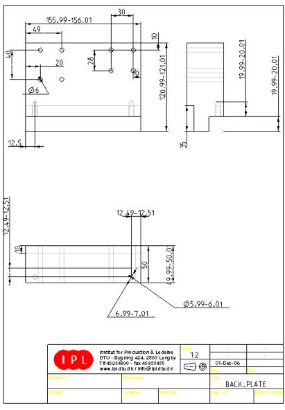
7.2.3 The back plate

 

 

            The plate in which the turntable rests must be mounted on the spindle and rail system. Mounting the turntable plate on a vertical back plate does this. The vertical back plate also serves as a linkage between the ball screw and rail system. A rectangular shaped aluminum block is used as support between the turntable plate and back plate. This block helps alignment of the turntable plate in the horizontal position.

 

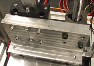
Figure 7.2.3.1 The back plate. The support block can be seen in the lower part of the picture.

 

 

 

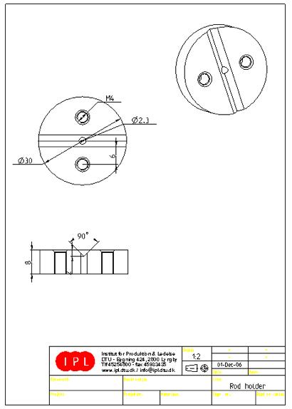
7.2.4 Reflector rod holder

 

            It is very important that the reflector rod is rotating in a plane perpendicular to the laser beam. This is achieved by fabricating a holder for the reflector rod with very tight tolerances.

 

            Fabrication itself demands that threads of varying diameters can be fastened to the holder. Also the material used for the holder must be very light to prevent a vast current drain as the motor is started. Finally it must be easy to machine. Obvious choice is aluminum alloy since its light weight and due to the machinability of the alloy.

 

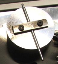
Figure 7.2.4.1 Reflector rod holder

 

            The holder is machined out of a solid aluminum rod. This rod will be turned with a lathe, which will machine it down to the specified dimensions in one clamping, to provide maximum rotational symmetry. A milling machine is used to cut a groove in which the reflector rod will be positioned and fastened.

 

 

7.2.5 The reflector rod

 

 

            The reflector rod may be interchanged with rods of varying in diameter due to the relation between rod diameter and resolution as explained in Chapter 6.4. What is of great importance is that it is as perfectly round as possible, and that the surface quality is as good as possible.

 

This can be achieved by extensive polishing of the surface or by surface treatment. The rod can be copper plated, or even plated with silver or gold. This enhances the rod in two ways. Foremost a material with good reflectivity can be plated to enhance performance at any given wavelength, and also a plating process will smooth out scratches and grooves on the surface of the rod. If the surface quality is so good that the scratches are below the wavelength of the laser they are not interfering with the reflected light^[17]. Such scratches are called subwavelength imperfections.

 

            A test has been conducted on a Wolfram rod with a diameter of 3 mm. This type of rod what is normally used as an electrode for TIG welding, and can withstand temperatures in excess of 3000˚C. It has a limited reflectivity at the wavelength of where 1075 nm where the test were conducted.

 

It was thought that the high melting point might rule superior to the reflectivity parameter. The reflectivity proved more important though. The laser simply began to cut grooves into the rod material. This can be seen on picture 7.2.5.1.

 

Picture 7.2.5.1 Cuts made by the laser beam in the Wolfram rod

 

            Experimental work has also shown that an ordinary aluminum rod seems to be good enough for the purpose of testing and validating the laser beam analyzer so an ordinary aluminum TIG filler rod will be used as reflector rod, and can easily be upgraded in future development.

 

 

 

 

7.2.6 The inverted T-frame skeleton.

 

 

            The frame must be strong, durable and most of all straight. Like the plane and the rod care must be taken when the frame is assembled to make sure it is straight. The best way of ensuring that the entire structure does not sway is to construct the base of the frame as a tripod. Hereby 3 points of the frame is in contact with the ground at any time.

 

            The frame itself is constructed in a standardized extruded aluminum profile system developed and produced by the German company, Bosch Rexroth. The profile is bought as one long extruded profile, and can then be cut to lengths that will be in the construction of the frame.

 

The profiles needed for the construction of the T-frame are listed in appendix 15.8 and are cut a few millimeters longer than the desired length. After that the last few millimeters are removed by milling them down to size. The milling process insures that the cut surfaces are perpendicular to the profile and when assembled the frame will be as straight as possible.

 

 

Figure 7.2.6.1 Bosch Rexroth profile system.

 

To make the assembly job easy, Bosh Rexroth sell prefabricated squared joints so that the frame can be assembled with only two bolts pr. joint. These joints come in different shapes and sizes so depending on the type of assembly it is possible to find a joint that suits the purpose.

 

 

7.2.7 Spindle and linear motion rail

 

 

            Vertical motion is made possible by using a ball screw and a linear rail system. These components are standard components and are readily available on the market. The ball screw and rail system that were utilized were unused part lying in the ILP/CALM laboratory and probably their origin is unknown. This is also the reason why the NC axis of the beam analyzer seems to be over-dimensioned.

 

            The rail system is used to stabilize the vertical motion and as a support for the back plate. This will ensure that there is no sideways slack in the system that can tilt the entire system to one side. The ball screw provides the system with a likewise vertical stability limited to the spindle slack.

 

            The ball screw has a 2.5 millimeters gradient. This means that by turning the ball screw 360 degrees one gets a horizontal movement of 2.5 millimeters. It is fastened to the frame by the means of two ball bearings in two flanged bearing housings.

 

 

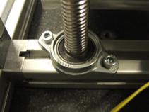
Figure 7.2.7.1 The bearing flanged housing

 

The advantage of such housings is that any misalignment between the ball screw and linear rail easily can be balanced out by the following routine. The ball screw and linear motion rail are loosely fixated on the back plate. The ball screw and rail are moved to the downmost position. The lower flanged housing are bolted tightly to the frame Then the spindle and rail system moved to the upmost position and the upper flanged housing are bolted tightly to the frame. Now the back plate are boltet tight and everything is aligned properly.

 

 

 

7.2.8 Strength of the turntable plane

 

 

            Since the final design of the beam analyzer is based on a free hanging plate it is important to investigate whether this construction will pose any problems related bending. The plate cannot during the experiment be allowed to bend downwards. Reason being that the plate is wanted to be perpendicular to the laser beam. Considering the design of the plate and its support, simple calculations can prove if the plate will bend and if it is a cause of worrying.

 

            The setup has been simplified into a situation for which there exist equations for bending and loading. The drawing bellow illustrates the situation in its simplified form.

 

 

 

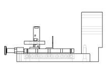
Figure 7.2.8.1 Loading situation for the plane where the arrow indicates the center and direction of the load force.

 

 

 

A set of equations from the classical beam theory can be used to calculate the bending under this type of loading^[18]. The load comes from the planes own weight and the weight from the turntable holding the instruments. So knowing the materials used in creation of the components it is possible to calculate the load using Newton’s second law of motion:

 

 

(Formula 7.2.8.1)

 

 

In this situation the acceleration is the force of gravity and the mass is mass of the turntable and plate system. In the worst case assumed that the plate and turntable will have a combined total weight of 5 kg. The force or load acting on the plate is then calculated to be 49.1 N.

 

The position of the load is usually put in the middle of the plate where the centre of gravity is assumed to be. However in this situation the loading will not occur in the middle. Reason being that the largest concentration of mass will be offset towards the end from the middle of the plate. Here it is very important to know all the dimensions.

 

The equations that describe the bending can be seen as formula 7.2.8.2. These equations are derived from beam theory, but can be applied in this case due to the fact that the plane acts as a beam, and the forces involved are not severe.

 

 

 

(Formula 7.2.8.2^[18])

 

Where index u is the bending in mm, the x is the position to where the bending on the beam is calculated, a is the position of the load measured from the support and L is the total length of the beam, or in this case the plane. E is the Young’s modulus and it is dependant on the material used. In this case the material used is aluminum with a Young’s modulus estimated to be 7.0 x 10⁴ N/mm². Index I is the moment of inertia of the plane. It is relative to the geometry of the plane. Since the plane has a rectangular shape its moment of inertia can be calculated as following:

 

(Formula 7.2.8.3^[18])

 

where t is the width of the beam and h is the height of the beam.

 

 

            The load situation from figure 7.2.8.1 can now be calculated. Formula 7.2.8.3 is first used to find the moment of inertia. The dimensions from technical drawings from the appendix 15.9 are used.

 

 

 

 

 

 

Now formula 7.2.8.2 is used to find the bending at far end of the turntable plate, where x=L=175 mm, as it is in this end the bending is greatest:

 

 

 

 

            It can be seen that the plate is found to bent 4.4 mm. This must be considered neglectable as the this is the bending at the very end of the plate. A dislocation of 4.4 mm of a plate with a length of 175 mm results in a bending angle so close to zero that any other manually aligned part of the system is expected to be more inaccurately aligned.

 

 

7.3 Electronics, mechatronics and software

 

 

7.3.1 The power supply.

           

            The power supply used to power all electronics is a standard ATX computer power supply rated to 150W. The voltages -12V, -5.0V, +5.0v and +12.0v can be drawn directly from the power wires of the power supply. An ATX power is not intended be turned on by the flick of a switch but from a signal from the motherboard of a computer. Fortunately it is easy to hot-wire the power supply by short-circuiting the power cable that is supposed to be attached to the motherboard. The crude paper-clip solution seen on picture 7.3.1.1 was only a temporarily solution until a proper on/off switch was put in place.

 

Picture 7.3.1.1 A hot-wired ATX power supply.

 

7.3.2 Stepper motor

 

 

The stepper motor used to drive the vertical axis had to be dimensioned. To make sure that a resolution of 1 mm can be met^{[Chapter 7]}, some calculations is required. Furthermore a set of equilibrium equations has to be solved to ensure that the torque of the stepper motor can turn the spindle.

 

The ball screw has the pitch of 2.5 mm/rev^{[Chapter 7.2.7]}. The stepper motor in consideration has a built-in gearbox at a ratio of 1:25 and a step length of 7.5 ˚ pr step^{[Appendix 15.5]}. Half-stepping is possible to this reduces the step length to the half

From these specifications it is possible to calculate the step length in vertical movement of the axis pr step:

 

 

The stepper motor fulfills the requirement for the resolution of the axis. The stepper motor comes in a product line of stepper motors that may be purchased with a range of different gearing ratios. If at a later point in time it becomes interesting to upgrade the resolution of the vertical axis, a stepper motor with a gearing up to 250:1 can be purchased ^{Appendix 15.5} and the resolution will then be a factor ten better.

 

The stepper motor is a low-torque stepper motor so even though it has a 1:25 gearing ratio it is needed to calculate if the stepper motor is powerful enough to turn the ball screw.

 

The following data is used for the calculations:

 

^[19]

 

 

Equilibrium equations, based on the unity circle, due to the fact that the motion of the ball screw is a rotation:

 

(Formula 7.3.2.1)

           

The friction between the balls in the ball screw and the spindle itself will also give a contribution to the system in form of a frictional force, which can be turned into torque by a simple equation:

 

        (Formula 7.3.2.2)

 

In the end a summation of the acting forces (torque) is needed to see the actual amount of torque present in the system:

 

 

 

When comparing this result to the torque that the stepper motor can deliver^{[Appendix 15.5]}, which is 0.731 Nm, it is seen that the stepper motor is suited for powering the vertical axis.

 

7.3.3 Stepper motor controller

 

 

A circuit board has been developed to control the stepper motor. Being a unipolar stepper motor, there are 6 wires protruding from the casing of the motor. Two of these wires are common ground wires, and the remaining four are input wires to four coils residing inside the stepper motor.

 

When current is applied over coil one to four, in a so-called stepper sequence, the stepper motor rotates 7.5 degrees per. Step, in one direction. By reversing the stepper sequence the stepper motor rotates the opposite direction.

           

The stepper motor controller is communicating through a serial port and is compatible with any computer, which has an RS232 based serial communications port.

 

A high-level communication method is used to interface to the stepper motor controller so that no programming skills or computer extensive computer knowledge is needed for direct interfacing with the controller. Communications can be set up with Hyperterminal, which is an application distributed with Microsoft Windows.

 

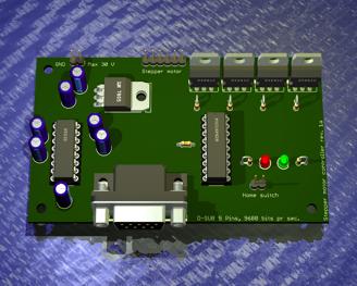
Figure 7.3.3.1 stepper motor controller board in a 3D view

 

 

 

 

The stepper motor controller can be divided into 3 subsystems.

 

1. A PIC16F628 processor, which runs a little ANSI C program. This program called the firmware communicates with a PC or other external device complying with the RS232 standard and drives and controls the stepper motor.

 

2. The MAX232 chip. On a PC a logical one equals positive voltage value up to 12 V and zero equals a negative voltage value down to -12V. On the PIC processor a logical one and zero equal respectively +5V and 0V. This chip converts logical ones and zeroes between the PIC processor and the PC.

 

3. A Darlington transistor array controlled by the PIC processor. This array consists of four TIP41C Darlington transistors and works as a valve-system opening and closing for current over the coils of the stepper motor.

 

 

Schematics for the electronic circuit can be found in appendix 15.3.

 

An overview of the execution of the firmware can be seen on the flowchart on chart 7.3.3.1. The source code to the firmware is available in appendix 15.4 and on the documentation CD-ROM, appendix 15.1

 

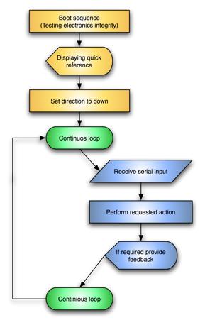
Chart 7.3.3.1 A flowchart of the PIC processor firmware.

7.3.4 Brushless motor and controller

 

 

The brushless motor, which drives the metal rod, has been found in the R/C hobbyist shop. It was the only motor that could be found that met both the geometrical restrictions that the analyzer as a whole should be no higher than 70 mm, and the requirements to the rotational speed^{[Chapter 7]}.

           

            Unfortunately purchasing the stepper motor and controller at an R/C hobbyist shop meant that no datasheet or specifications could be retrieved. It was just told that the brushless motor was capable of a rotational speed in excess of 40,000 RPM.

 

This was a reason of concern. The brushed DC motor used for the initial work did not only have problems in relation to rotational speed, it was also poorly balanced causing vibrations. This could be seen on the background noise of the detector signal.

 

A measurement of background noise on the detector signal of the experimental setup from chapter 6 was used to examine if the new motor was any better than the old motor in relation to balancing. The results of the analysis is seen in figure 7.3.4.1. The brushless motor was remarkably better balanced.

 

Graph 7.3.4.1 The background noise for the old DC motor and the new brushless motor.

 

 

Brushless motors do not just operate by the means of a DC current. They need two auxiliary bits of electronics. The one being a speed controller and the other is a square signal generator.

 

A brushless motor is best described as a brushed motor turned inside out. A permanent magnet is fixed to the rotor and two coils which are fixated to the stator. Just the opposite of what is seen on a traditional brushed motor. Each coil is turned on in sequence to create a magnetic field so that the permanent magnet on the rotor turns a partial revolution.

 

By controlling the frequency of the sequence the speed of the brushless motor can be accurately controlled. This is done by the speed controller.

 

An R/C based speed controller needs an input signal to operate. This signal is a square signal sent to the speed controller as a pulse train. The pulse period is 50 Hz and it is the width of the on-time that determines the speed of the motor. The longer the on-time, the greater the speed. This is illustrated in the figure 7.3.4.1

 

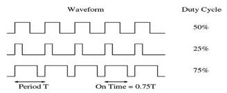
Figure 7.3.4.1 Visualization of the wave form VS. duty cycle

 

The pulse train is generated by the second piece of auxiliary equipment, a so-called multiplexer. It is based on analogue electronics and a 555-timer IC, which is a timer chip capable of generating the pulse train.

 

7.3.5 Beam analyzer controller software:

 

 

The beam analyzer software interface is a Win32 based application programmed in Microsoft Visual Studio. The software consists of four different parts.

 

1. A Communications part, where serial communication with the stepper motor board is established.

 

2. A Picoscope interface part, where a window-hook to the Picoscope software is established.

 

3. A data acquisition part where a dumping routine that grabs data from the Picoscope and dumps the data to the hard drive of the PC.

 

4. A manual control part where the user can take control over the beam analyzer axis.

 

 

 

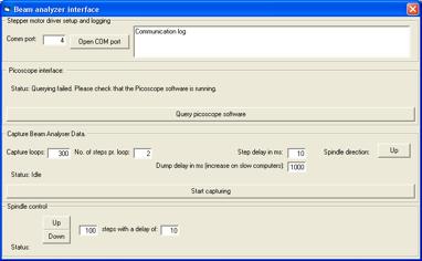
Figure 7.3.5.1 The beam analyzer Win32 controller software

 

The Picoscope software is distributed with a dynamic link library, a so-called .DLL file. This library makes it possible for software developers to interface to the Picoscope.

 

Unfortunately the sampling rate of a continuous streaming of data from the Picoscope trough the USB cable to the computer is way to slow to meet the requirements for sampling of the data from the detector of the laser beam analyzer.

 

Another operation mode called block mode is based on the utilization an on-board memory stack on the Picoscope. This means that a little memory bank inside the scope captures data in real time, and this memory buffer can be dumped to the computer.

 

By using the block mode it is hereby possible to retrieve small pieces real time sampled data, with a higher sampling rate from the Picoscope, than when the Picoscope are run in continuous stream mode.

 

Unfortunately all the advantages of direct interfacing trough the .DLL are lost by using the block mode. This is mainly due to the fact that a trigger point has to be set for the scope to operate in block mode. This is very difficult for the user to do without a good graphical interface, and such interface is a major task to develop.

 

This leaves another option. To make a graphical user interface hack, abbreviated to GUI hack. This is done by letting the user set a trigger point in the Picoscope software as one would do when the Picoscope software are used as a stand-alone application.

 

When the trigger point is set, the beam analyzer software is activated. The beam analyzer software scans the processes running on the computer and identifies the Picoscope software. After that it starts to send emulated keyboard strokes to take control over the Picoscope software, acting as if a user was interacting with the Picoscope software.

 

Now the Beam analyzer software copies data from the Picoscope software to the clipboard of the computer. Afterwards the data of the clipboard are manipulated and streamed to the hard drive of the computer.

 

 

 

The data grabbing routine is visualized in chart 7.3.5.1.

 

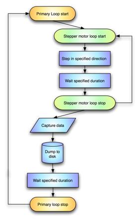
Chart 7.3.5.1 Flowchart over the Win32 software

 

7.3.6 REV counting mechanism

 

 

A REV counting mechanism has been added to the construction to be able to precisely determine the rotational speed of the reflector rod. This mechanism is based on a slotted optocoupler. The optocoupler has two section. One section contains an IR LED, and another section contains an IR sensitive photo detector. The slot between these two components is just exactly wide enough to allow the rod to pass trough as it rotates. Every pass of the rod will interrupt the light from the IR LED passing through the slot towards the photo detector. This will trigger a signal that can be monitored on the oscilloscope. An overview of the optocoupler can be seen in figure 7.3.6.1.

 

 

 

Figure 7.3.6.1 Optocoupler schematic

 

 

The optocoupler used in the beam analyzer is placed on a small circuit board with some auxiliary resistors, and is powered from the common power supply. The board is designed in such manner that it is possible to directly attach two signal wires to the secondary input of the oscilloscope that are used to monitor the detector and hereby provide precise rotational feedback.

            It was of interest to examine how precise the revolutional speed could be monitored. For this, an analysis of the optocoupler fall time was analyzed.

 

Graph 7.3.6.1 Fall time of the optcoupler.

 

A worst case scenario of the deviation of the trigger signal was calculated. Assume that the motor is rotating at 18000 rev/min = 300 rev/s. This means that one revolution takes 1/300 second.

 

Triggering on the noise to the right of the end of the slope of the optocoupler is of concern As seen on graph 7.3.6.1, the noise fades out at 200 ns. A safety margin is set so noise is assumed to be possible to occur up to 500 ns after the actual optocoupler signal. 500 ns = 5.0e-7 seconds. Now the deviation in percent is calculated:

 

 

This again can be converted to a deviation in rotational speed to 270 RPM which can be neglected with no noticeable affects during post processing.

8. The finished laser beam analyzer

 

Picture 8.1 shows an overview of the finished laser beam analyzer. The arrows point out the different sub-systems on the analyzer frame and of the electronics.

 

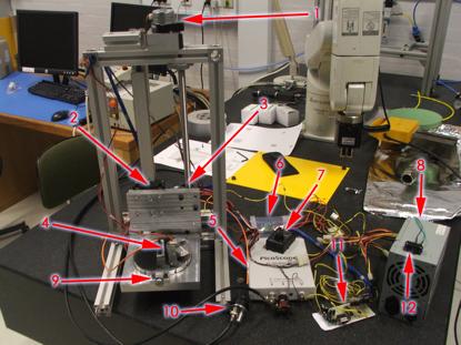Picture 8.1 An overview of the beam analyzer. 1. The stepper motor with built in gearbox, 2. The linear rail sledge, 3.The ball screw, 4. The turntable with subcomponents, 5.The Picoscope USB oscilloscope., 6. The speed controller for the brushless motor, 7. The multiplexer for the speed controller, 8. The power supply 9. The indexing bolt for the turntable, 10. The detector, 11. The stepper motor, 12.The on/of switch to the entire system.

 

Picture 8.2 provides a close-up picture of the turntable itself where ann overview of the sub components of turntable are visible:

 

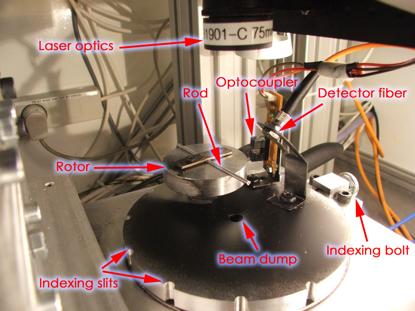
Figure 8.2 An overview of the sub components of the turntable

 

 

9. Economic overview

 

 

There have been developed an economic overview of the costs involved in the development of the laser beam analyzer. This can be found in appendix 15.8. The overall costs for the development was 5070,- DKR. Which is approximately 875$ USD.

 

10. Validating the laser beam analyzer

 

 

As a proof of the integrity of the finished laser beam analyzer a test series has been conducted. These tests were carried out nearing the end of the project and unfortunately due to lack of laboratory time thorough testing of the laser beam analyzer has to be done by its heritors.

 

 

10.1 Measurement set 1

 

 

One test series has been performed at which beam propagation has been measured for falling power setting starting from maximum power and falling with 500 mA. The series gives an impression of enhanced data density and hereby resolution of the beam propagation. The M² and beam waist is also expected to be roughly the same throughout the datasets

 

10.1.1 Measurement data 6A:

 

The first dataset was captured with the beam analyzer with the fiber laser set to 6A/20W output. The 2D plot of the raw measurement data clearly visualize the extended data density.

 

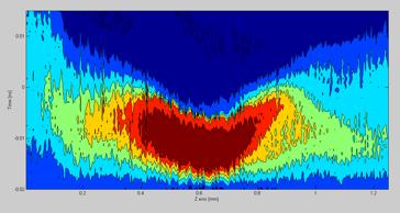
Graph 10.1.1.1 Raw source data at 6A

 

The intensity distribution in the data seems to be distorted. The plot seems to arch downwards. This is expected, and the explanation to this phenomenon is to be found in the Picoscope software and is related to the trigger point. The trigger pint determines the start point at which data is captured. Lets look at what happens

 

 

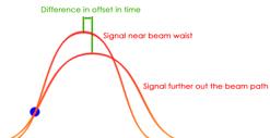
Figure 10.1.1.1 Relation between time offset and trigger point

 

As figure 10.1.1.1 shows, the time at where the maximum of the scope signal will be found has a larger offset in time from the trigger point far from the beam waist than what will be found close to the beam waist. This causes the distortion and since the raw data is fitted with the Gaussian fitting algorithm and normalized this effect is zeroed out. Unfortunately this effect makes it impossible to determine any beam defect related to e.g. alignment but can be ruled out by triggering on the optocoupler signal instead of the intensity signal. This has not been done in the test series due to limitations in the sampling range of the Picoscope hardware. A better oscilloscope as well as moving the optocoupler closer to the measuring point will make this possible.

 

The source data was also analyzed in 3D since this visualization gives a better impression of how much noise there is on the signal and gives a more depth-like visualization. A smoothing algorithm is used to remove the noise on the signal so that even more details become visible.

 

 

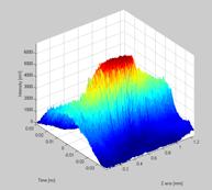
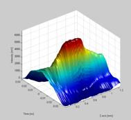
Graph 10.1.1.2 A 3D visualization of the raw data

 

Finally the beam propagation path is calculated from the raw data. This is seen in figure 10.1.1.3

 

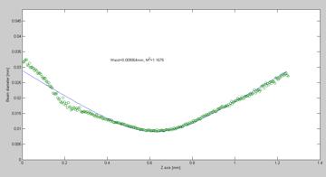
Graph 10.1.1.3 Beam propagation path of the beam

 

First and foremost it is seen that the fitting algorithm performs much better with the high density raw data compared to what was seen in the initial experiments. In the left part of the beam propagation path it is seen that there seem to be some signal distortion. This is the focusing side of the beam path and an explanation of this behavior is yet to come.

10.1.2 Measurement data at 5.5A

 

The second dataset show in general the same tendencies as the first one. Figures of the 2D/3D raw data plots shows this.

 

 

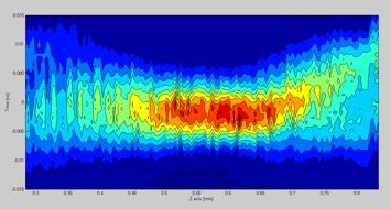
Graph 10.1.2.1 A 2D plot of the raw data at 5.5A

 

Unfortunately the same tendency with noise on the focusing side of the beam path was seen. The noise was so bad that the data points closest to the focusing lens had to be filtered away in order to make a decent beam propagation path.

 

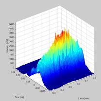
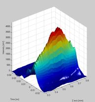
Graph 10.1.2.2 A 3D visualization of the raw data

It is seen visible that the raw data has been trimmed.

 

 

 

The beam propagation path of the fitted and trimmed raw data is shown in figure 10.1.2.3. The noise on the left side of the beam path is still visible

 

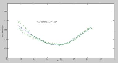
Graph 10.1.2.3 The beam propagation plot at 5.5.A

 

10.1.3 Measurement data at 5A

 

A new distortion pattern in the raw data is seen in the third data set. This is again due to the trigger signal.

 

 

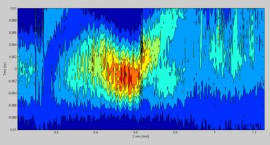
Graph 10.1.3.1 A 2D visualization of the raw data.

 

This distortion pattern has two major shear lines at the values Z ≈ 0.16 and Z ≈ 0.62. These shears are due to the fact that the operator had to adjust the Picoscope trigger point twice during the experimental procedure in order to keep triggering on the signal. This again is of no influence since the offset in time is normalized in the post processing procedure.

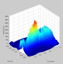
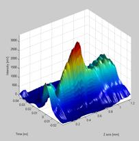
Graph 10.1.3.2 A 3D visualization of the raw data. The signal distortion is extensive in the right side of the plots.

 

The third and final beam propagation plot, figure 10.1.3.3, shows the same defects as the first series. The defects seems to be systematic.

 

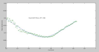
Graph 10.1.3.3 Beam propagation plot at 5A

 

The varying power settings of the 3 measurement sets should not affect the M² and waist in a extensive degree. A mean beam waist and M² can therefore be calculated:

 

 

The same calculation can be performed for the beam waist as it is assumed that it will not be affected in any major degree by the differing laser output power:

 

 

10.2  Conclusion of the validation experiments

 

Though a distortion pattern seemed to be consistent through all 3 measurements it has been shown that the laser beam analyzer has the potential of providing consistent data with low deviation as seen around the beam waist and in the right side of the beam propagation plots. Even though M² and the beam waist seemed to be similar in the 3 measurement series one should keep in mind that the fitting algorithm that calculates M² and beam waist is affected by the distorted signal.

 

The true cause of the distortion has not been found but there are two theories that might give an explanation of why it is so.

 

The first theory visualized in figure 10.2.1 is based on two factors. These are defects in the surface of the reflector rod combined with a misalignment of the laser optics. If it should be so that these two events occur at the same time, a defect might cause distorted reflections in one end of the measurement series but as the reflector rod is moved vertical through the beam path the misalignment of the optics will cause the laser beam spot get nudged across the surface of the reflector rod for each step in the vertical direction and hereby move away from the defect.

 

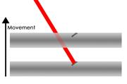
Figure 10.2.1 A distortion phenomenon theory

 

 

 

Another theory could is that the reflector rod gets damaged by the laser. It is clearly visible that raw data from measurement 1 is purest and measurement 3 is the most distorted. This could be due to the changes in power setting but might be an indication of the deteriorating state of the reflector rod throughout the experiment.

 

10.3 Hunting the distortion problem.

 

No true explanation of the distortion problem had been found throughout the first set of experiments on the beam analyzer. Another experiment was conducted to see if the pattern was consistent. The reflector rod was changed. The laser beam analyzer was removed from the laser cabinet, and then aligned again. Only one set of measurements was carried out. The results of these were surprising though.

 

 

 

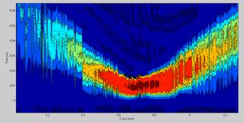
Graph 10.3.1 The 2D raw source data looks promising.

 

The 2D plot of the source data looks nice. There seem to be consistency in the measurement data. A minor triggering instability is seen in the start of the data series. That is the data in the left part of the screen. This is most likely caused by the triggering phenomenon that was discussed in chapter 10.1.1.

 

The 3D graphs of the source data seen in Graph 10.3.2 looks just as promising. The area close to the beam waist seen as the area that peaks with the read color is not centered in the graph. Therefore the graphs cheat the eye so that it looks asymmetrical. Actually the data seem to be more or less symmetrical on either side of the waist area, it is just so that there are more measurement point on one side of the focal point than the other. The symmetry is good news. There are no sign of the distortion phenomena whatsoever.

 

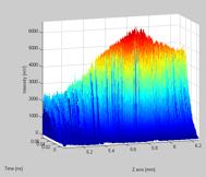
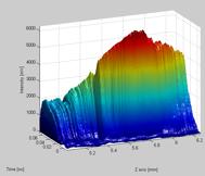
Graph 10.3.2 The 3D raw source shows no sign of distortion.

 

 

            Finally the beam propagation calculations are carried out. The data was trimmed a bit so that the beam waist is placed in the center of the graph. This was solely done to aid the fitting algorithm in making a good fit.

           

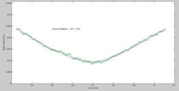
Graph 10.3.3 A good fit with no distortion to be seen.

 

            As seen from Graph 10.3.3 the distortion phenomenon has completely disappeared. It seemed that it for reasons unknown helped to start over and realign the beam analyzer again. This favor the theory proposed in chapter 10.2 relating to a misaligned optical system combined with surface defects on the reflector rod. Though the phenomenon must be examined further before conclusions can be made, this might just prove to be the right theory.

 

11. Error identification

 

Many errors can occur while performing a beam analyzing experiment. Some of these errors such as reflector rod damage and aligning has been explained in the previous chapter, 6.18. Some other causes of error that was actually encountered during the experimental work is listed below.

 

11.1 Human errors

 

The experiments gave an overview of what type of problems could occur when operating the laser beam analyzer. Even though there was focus on minimizing the human factor when the laser beam analyzer was constructed, it has show that human error still can occur. As an example is what happened in experiment 10.1.3. There the operator set the trigger point on the oscilloscope incorrectly. Though this error looked critical when the raw source data is examined it was easily be corrected in the post processing procedure as the time axis is normalized.

 

11.2 Reflector rod

 

            The reflector rod is another possible cause of error. It can be misaligned; the laser can damage it, the quality of the rod can be to poor, or it can simply just be dirty, all things which causes distorted reflection. The length of the free hanging rod is also important. If the free part is too large the rod can flex and the angle to the detector signal is no longer valid.

            Vibrations from a misaligned reflector rod can cause problems normally seen as random background noise.

 

11.3 Rotational speed

 

            The rotational movement of the rod itself is of importance. The rise and fall time of the detector/oscilloscope can prove crucial in the quality of the results. If the rotational speed is too great the detector will simply not be able to discharge the fast enough.

 

 

 

 

 

11.4 Cladding mode

 

Another problem that was encountered is what is known as cladding mode. This concerns the fiber that collects the reflected light from the reflector rod and relays the light to the detector. What happens is that some or all of the light traveling inside the fiber traveling in the cladding layer of the fiber instead of the core. The cladding has a higher refractive index than the surrounding outer polymer coating meaning that if the angle of incidence of the light entering the fiber is to large then the light might get trapped in the fiber. The way to prevent this to occur is to ensure that the detector fiber is close of to the reflected beam. Simply said Snell’s law must apply.

 

(Formula 11.4.1)

 

 

Where n1, n2 are the reflective indexes of the transition layers and q₁ , q₂ are the interaction angles.

 

If cladding mode should occur then the mode coming out of the collector fiber and into the detector will be for the mode called TEM10^[20]. This can be seen on the Picoscope as a triple-peak as in figure 11.4.1

 

 

 

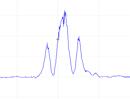
Figure 11.4.1 Left: TEM10 mode Right: The corresponding Picoscope output.

12. Conclusion

 

A long forgotten but promising beam analyzing method from 1983 has been revalidated and ported to a version that is suited for numerical autonomous data collecting and data processing

 

The hardware platform for a laser beam analyzing device has been developed and built.

 

The electronics and mechatronics to control the beam analyzing device has been developed and built.

 

A software platform for the beam analyzing platform consisting of an embedded stepper motor controller firmware, an NC control interface and an interface for the Picoscope software has been developed.

 

A data collecting routine has been programmed so that beam analysis data can be captured autonomous at a rate more than 600 percent faster than what is possible to do manually.

 

A numerical post processing script has been developed that can be used to process the measurement data, and estimate a beam propagation path with related beam propagation parameters.

 

All these subsystems as been assembled into one unit being the laser beam analyzer

 

The laser beam analyzer has been experimentally verified and fulfills the demands requested from the IPL/CALM group as well as the demands set by the authors to accommodate the demands defined during the initial experimental work.

 

The laser beam analyzer platform and underlying theory has been documented and reported based on literature and insight into laser theory and optics obtained from the personnel of the IPL/CALM group.

 

13. Future work

 

Beam analyzing is a complex science in itself. That fact that a leaser beam analyzer has been built and that it has been validated through a series of experiments does not mean that the finish line is just around the corner. It would be more appropriate to say that we have been given a good starting point to really examine the possibilities of beam analyzing. This starting point is in the form of a good platform that allows students and staff at IPL/CALM to perform further experimental work in the field of beam analyzing.

 

A vast parameter space determining the resolution of the laser must be sought. A just as overwhelming job of calibration of the beam analyzer must be undertaken. Routines for the use of the equipment must be defined, and many systems can be upgraded over time.

 

Work that is of immediate interest to examine further is:

 

-       How can the resolution of the beam analyzer be determined experimentally?

-       How does different reflective coatings improve the reflector rod?

-       How can the data post processing script be expanded to handle a true 3D analysis?

-       How can the reflector rod and fixture be balanced better?

-       How can the optcoupler system be tuned so that trigging on the optcoupler works better?

-       How can the physical dimensions of the beam analyzer be optimized?

-       Should a more sturdy skeletal frame be built?

-       Should the resolution of the vertical axis be improved?

-       Should a fast rising rectifying diode array to protect the stepper motor controller from inducted voltage surge be incorporated in the controller?

 

…and the list goes on. A beam analyzer platform has been built, and the possibilities for further development of the beam analyzer are of tremendous proportions. It is now up to the creative mind of the engineer to determine how the analyzer platform shall be mould to perfection

 

 

14 References

 

[1]        Lim G.C. and Steen W.M, Laser beam analyzer, Dept. of Metallurgy 1983, Imperial College, London SW7, GB

 

[2]        W.M Steen, Laser material processing, third edition chapter 10.2 and 10.2.1

 

[3]        W.M Steen, Laser material processing, third edition chapter 3

 

[4]        W.M Steen, Laser material processing, third edition chapter 2.8.1.1

 

[5]        http://www.rp-photonics.com/beam_waist.html

 

[6]        http://www.rp-photonics.com/rayleigh_length.html

 

[7]        W.M Steen, Laser material processing, third edition chapter 2.6

 

[8]        W.M Steen, Laser material processing, third edition chapter 2.8.1

 

[9]        http://www.rp-photonics.com/m2_factor.html

 

 

[10]      W.M Steen, Laser material processing, third edition figure 2.14

 

[11]      http://www.rp-photonics.com/gaussian_beams.html

 

[12]      www.koheras.com, model HPM15

 

[13]      W.M Steen, Laser material processing, third edition chapter 2.9

 

[14]      http://en.wikipedia.org/wiki/Optical_coating

 

[15]      http://en.wikipedia.org/wiki/Gaussian_function

 

[16]      W. M. Steen, Laser Material Processing, Third edition, formula 2.15

 

[17]      http://www.optics.arizona.edu/masud/OPN_Engineering.pdf

 

[18]      Bjarne Christian Jensen, Teknisk ståbi, 19 udgave, Erhvervsskolernes forlag

 

[19]      www.designnews.com/article/CA435593.html

 

[16]      W. M. Steen, Laser Material Processing, Third edition, page 82

 

15 Appendices

 

 

15.1 The documentation CD-ROM

 

As a part of the appendix material is a ISO formatted CD-ROM. This CD-ROM contains all program source code for the stepper motor controller, the Win32 application and the matlab script. It also contains CAD drawings and PDF datasheets for vital components.

 

15.2 Matlab script

 

 

Script source for matlab calculations. Two primary script files are used. There ase Gauss_fit.m and beam_propagation.m. Gauss_fit.m contains the algorithm that makes Gaussian fits of source data from the Picoscope and beam_propagation.m calculates the beam propagation parameters.

 

15.2.1 Gauss_fit.m

 

Gauss_fit.m is the file that is the one of the ma

 

CLOSE ALL;

clear all;

set(0,'DefaultFigurePaperType','A4');

global lambda

 

 

%initial setting

lambda = 0.001075; %wavelength

filename = 'output.txt' %name of data file

speed = 5.388; % ms/rotation (time between two peaks)

measuringdist = 33; %Distance at which the measurements take place.

 

inputfiles = 300; %Number of inputfils

steplength = (2.5/1200)*2 %stepsize times number of steps

%reading of data

rawdata=fun_load_data(inputfiles);

 

for ssk = 1:inputfiles

 

if (ssk==1)

zdata = ssk*steplength;

end

zdata = [zdata,ssk*steplength];

end

 

 

%numbers of datasets

[row col]=size(rawdata);

 

%saperating and sorting rawdata into two, time, and intensity

[z_new_data,t_new_data,i_new_data]=fun_sort_data(zdata,rawdata);

 

 

 

%fitting the gauss curves

for j = 1:col/2;

%Bredde=data(:,j).*Hastig*1e-9;

%finding the peak for start

omkreds = 2*pi*measuringdist; %mm

hastighed = omkreds/speed;

tt_new_data(:,j)=t_new_data(:,j).*hastighed*1e-6;

 

%hold on

[value, colno]=max(i_new_data(:,j));

b1=value;

b2=0.1;

b3=tt_new_data(colno,j);

b4=0;

beta=[b1 b2 b3 b4];

%fitting

peak_data = nlinfit(tt_new_data(:,j),i_new_data(:,j),@fun_gauss,beta);

peak_data_2 =nlinfit(tt_new_data(:,j),i_new_data(:,j),@fun_gauss,peak_data);

peak_results(j,1)=z_new_data(1,j);

for i=2:5

peak_results(j,i)=peak_data_2(i-1);

end

%null the time axes

t0_new_data(:,j)=tt_new_data(:,j)-peak_results(j,4);

end

 

%plotting all in one with offset

%offset = 300;

%for j=1:col/2

% off_i_new_data(:,j)=i_new_data(:,j)+j*offset;

% off_y(:,j)=fun_gauss(peak_results(j,2:5),tt_new_data(:,j))+j*offset;

%end

%plot(t0_new_data,off_i_new_data,t0_new_data,off_y)

%xlim([(-3*max(peak_results(:,3))) 3*max(peak_results(:,3))])

 

 

 

 

 

%poltting a 3D graph of the beam propagation

figure

contourf(z_new_data.',t0_new_data(:,1),i_new_data)

Ylim([(-1*max(t0_new_data(:,1))) 1.5*max(t0_new_data(:,1))])

 

 

xlabel('Z axis');

ylabel('Time');

zlabel('Intensity');

 

 

upperoffset_y=170

loweroffset_y=260

 

figure

%meshc(z_new_data.',t0_new_data(:,1),i_new_data)

mesh(z_new_data.',t0_new_data(upperoffset_y:loweroffset_y,1),i_new_data(upperoffset_y:loweroffset_y,:))

%Ylim([(-1.5*max(t0_new_data(:,1))) 1.5*max(t0_new_data(:,1))])

%surf(z_new_data.',t0_new_data(upperoffset_y:loweroffset_y,1),i_new_data(upperoffset_y:loweroffset_y,:),'LineStyle','none')

 

xlabel('Z axis');

ylabel('Time');

zlabel('Intensity');

 

%saving data, old filename, data to be saved, add on to filename

save_data(filename, peak_results, 'gauss_fit_');

 

15.2.2 beam_propagation.m

 

 

            CLOSE ALL;

clear all;

set(0,'DefaultFigurePaperType','A4');

global lambda

 

 

%initial setting

lambda = 0.001072; %wavelength

filename = '3d_old_motor.txt' %name of data file

beam_para_guess = [0.001 1.2 1.5]; % start guess on [waist(mm) M2 z-position (mm)]

speed = 9.7; % s/rotation (time between two peaks)

 

%inport data from saved file

data=load_save_data(filename,'gauss_fit_');

 

 

%beampropagation

%direct fitting

beam_prop_direct = nlinfit(data(:,1), abs(data(:,3)),@fun_beam_direct, beam_para_guess);

beam_prop_direct2 = nlinfit(data(:,1), abs(data(:,3)),@fun_beam_direct, beam_prop_direct);

 

 

%therytical curves

x=min(data(:,1)):0.01:max(data(:,1));

 

y_direct=fun_beam_direct(beam_prop_direct2,x);

 

 

plot(x,y_direct,data(:,1)...

,abs(data(:,3)),'o')

ylim([0 1.5*max(abs(data(:,3)))])

 

 

text(max(x)/3,1*max(abs(data(:,3))),strcat(strcat('Waist=', num2str(beam_prop_direct2(1))), strcat(' M^2=', num2str(beam_prop_direct2(2)))) )

%teta=[1 0 0];

%beam_fit_ISO = nlinfit(header,(2*results(:,2)).^2,@fun_beam_ISO,teta);

%Waist=sqrt(beam_fit_ISO(1)-(beam_fit_ISO(2).^2/(4*beam_fit_ISO(3))))/2;

 

%M2=(pi*sqrt(beam_fit_ISO(1)*beam_fit_ISO(3)-(beam_fit_ISO(2)^2)/4))/(4*lambda)

%Z0=-beam_fit_ISO(2)/(2*beam_fit_ISO(3));

%Zr=sqrt(beam_fit_ISO(1)*beam_fit_ISO(3)-beam_fit_ISO(2)^2/4)/beam_fit_ISO(3);

 

15.2.3 Support functions for the matlab script

 

When the matlab script is executed it will call many sub modules and scripts. These script files are due to their sized appended to the report in a digital media in form of the documentation CD-ROM, appendix 15.1

 

15.3 Stepper motor controller schematics

15.4 Stepper motor controller firmware code

 

// ###################################################

// # #

// # This code is written for the CCS C Compiler #

// # /Coding by David #

// ###################################################

#include <16F628.h>

#include <math.h>

#include <stdlib.h>

#fuses INTRC, NOLVP, NOWDT, PUT, BROWNOUT

 

#use delay(clock=4100000)

#use rs232(baud=9600,parity=N,xmit=PIN_B2,rcv=PIN_B1)

 

 

 

main() {

char theanswer;

char UPDATELED;

int thedir;

int bootno;

int stepno;

 

bootno = read_EEPROM (1);

bootno++;

write_eeprom(1,bootno);

printf("Booting Stepper motor driver v. 0.1b...\n\r"); // send alive message

printf("This is boot no. %d.\n\r",bootno);

printf("Performing LED tests...\n\r");

 

 

output_high(PIN_B4);

delay_ms(200);

output_high(PIN_B7);

delay_ms(200);

output_low(PIN_B4);

delay_ms(200);

output_low(PIN_B7);

 

printf("LED tests sucessfull.\n\r\n\r");

printf("All systems running. Ready to accept commands.\n\r");

printf("\n\r");

printf(" -= Made by s031950 and s011480 =-\n\r");

printf("\n\r");

printf("\n\r");

printf("\n\r");

 

printf("Quick reference:\n\r");

printf("Set the direction of movement by sending a d- or u-character.\n\r");

printf("Start the seek home procedure by sending a h-character.\n\r");

printf("send a 1-character to initiate a step in the current direction.\n\r");

 

printf("\n\r");

printf("\n\r");

printf("\n\r");

printf("Direction is changed to: down\n\r");

// port_b_pullups(TRUE);

 

stepno =1;

thedir = 1;

port_b_pullups(TRUE);

while(true) {

 

theanswer = GetCh();

 

 

 

 

 

if(theanswer=='d'){

 

thedir = 1;

printf("Direction is changed to: down\n\r");

 

}else if(theanswer=='u'){

 

thedir = 0;

printf("Direction is changed to: up\n\r");

 

}else if (theanswer == '1'){

 

//this is a step pulse

 

if(thedir==1){

 

stepno = stepno + 1;

 

if(stepno == 5){

stepno=1;

}

 

}

 

 

if(thedir==0){

 

stepno = stepno - 1;

 

if(stepno == 0){

stepno=4;

}

 

}

 

if( input(PIN_B3) == 0 || thedir == 0){ //if-or statement for at forhindre at k¯re ned nÂr home er nÂet.

 

if(stepno ==1){

OUTPUT_HIGH(PIN_B4);

OUTPUT_LOW(PIN_B5);

OUTPUT_LOW(PIN_B6);

OUTPUT_LOW(PIN_B7);

}else if(stepno ==2){

 

OUTPUT_LOW(PIN_B4);

OUTPUT_HIGH(PIN_B5);

OUTPUT_LOW(PIN_B6);

OUTPUT_LOW(PIN_B7);

 

}else if(stepno ==3){

 

OUTPUT_LOW(PIN_B4);

OUTPUT_LOW(PIN_B5);

OUTPUT_HIGH(PIN_B6);

OUTPUT_LOW(PIN_B7);

 

}else if(stepno ==4){

 

OUTPUT_LOW(PIN_B4);

OUTPUT_LOW(PIN_B5);

OUTPUT_LOW(PIN_B6);

OUTPUT_HIGH(PIN_B7);

}

}

 

 

 

}else if (theanswer == 'h'){

 

//this is a step pulse

printf("Seeking home\n\r");

thedir = 1;

 

while( input(PIN_B3) == 0){

 

 

OUTPUT_HIGH(PIN_B4);

OUTPUT_LOW(PIN_B5);

OUTPUT_LOW(PIN_B6);

OUTPUT_LOW(PIN_B7);

delay_ms(3);

 

OUTPUT_LOW(PIN_B4);

OUTPUT_HIGH(PIN_B5);

OUTPUT_LOW(PIN_B6);

OUTPUT_LOW(PIN_B7);

 

delay_ms(3);

 

OUTPUT_LOW(PIN_B4);

OUTPUT_LOW(PIN_B5);

OUTPUT_HIGH(PIN_B6);

OUTPUT_LOW(PIN_B7);

 

delay_ms(3);

 

OUTPUT_LOW(PIN_B4);

OUTPUT_LOW(PIN_B5);

OUTPUT_LOW(PIN_B6);

OUTPUT_HIGH(PIN_B7);

 

delay_ms(3);

}

printf("Home reached\n\r");

}

 

 

 

 

//HHHHHHHHHHHHHHHHHHHHHHHHHHHHHHHHHH

}

 

 

}

 

 

 

 

 

 

15.5 Stepper motor data sheet

 

15.6 Detector datasheet

 

 

15.7 SKF 61819 ball bearing datasheet

 

 

 

15.8 Parts and costs

 

				Parts mechanics:
Reseller	Item no.	Amount	Unit	Description	Unit price (DKR)	Total price (DKR)
				Motors
RS Online	351-4625	1	stk	Unipolar 25:1gear 7.5deg steppermotor,5V	328.75	328.75
Holte modelhobby		1	stk	Brushless motor incl styring	1200	1200
				Standard profiles
Bosch Rexroth		2	stk	30x30x210 rexroth profile
Bosch Rexroth		2	stk	30x30x100 rexroth profile
Bosch Rexroth		3	stk	30x30x156 rexroth profile
Bosch Rexroth		2	stk	30x30x400 rexroth profile
				6 meter purchased at 350 DKR/meter:	2100	2100
Bosch Rexroth		6	stk	30X30 rexroth corner	>500	500
				Bearings
www.danskkuglelejecenter.dk		1	stk	SKF no. 61819 without seals	750	750
				Parts stepper motor controller:
	Elsupply Item No.	Amount	Unit	Description	Unit price (DKR)	Total price (DKR)
www.elsupply.dk	7612	1	plade	One sided photoprint, 160x100 mm	21.6	21.6
www.elsupply.dk	5514.2	6	stk	2 poled wireclips	2.4	14.4
www.elsupply.dk	40PIC16F628-20/P	1	stk	PIC16F628 el. Pinout, and clock kompatibel processor	36.3	36.3
www.elsupply.dk	41533	1	stk	33 kohms resistor. 1 piece used. Comes in bundles of 100	15	15
www.elsupply.dk	4510	1	stk	red 5 mm LED	0.71	0.71
www.elsupply.dk	4511	1	stk	green 5 mm LED	0.71	0.71
www.elsupply.dk	41333	1	stk	330 ohms resistor. 2 pieces used. Comes in bundles of 100	15	15
www.elsupply.dk	6003RØD	1	stk	On/off switch	3.48	3.48
www.elsupply.dk	6509.06	6	stk	U cooling plate	2	12
www.elsupply.dk	21108	1	stk	RADIAL ELEKTROLYT 4700µF-16V	8.34	8.34
www.elsupply.dk	21109	1	stk	10uf elektrolyt capacitor	0.66	0.66
www.elsupply.dk	21125.8	1	stk	0,1 uf capacitor	1.14	1.14
www.elsupply.dk	2827805	1	stk	LM78L05 el similar 5V voltage regulator	2.76	2.76
www.elsupply.dk	25P600B	1	stk	rectifyer diode 6A / 100 volt	4.74	4.74
www.elsupply.dk
www.elsupply.dk	41356	1	stk	560 ohms resistors. 4 piece used. Comes in bundles of 100	15	15
www.elsupply.dk	30TIP41C	4	stk	TIP41C NPN darlington transistors	7.14	28.56
www.elsupply.dk	40MAX232C	1	stk	Max232 serial interface
www.elsupply.dk	21125.8	5	stk	0,1 uf capacitor	1.14	5.7
www.elsupply.dk	5451	1	stk	D-SUB female 9PL.90gr.with 90 deg. bend	5.39	5.39
					Grand total:	5070.24

 

15.9 Technical drawings

15.9.1 Turntable overview

15.9.3 Back plate

 

 

15.9.3 Turntable plate

15.9.4 Reflector rod fitting

 

15.9.5 Turntable

 

 

15.9.6 Detector holder

 

15.9.7 Indexing bolt fitting

 

15.10 Optocoupler holder

 

 

15.9 Tolerance chart